An Interview with Prof. L. Randall Wray

1- Historically, it seems the financial capital has a second wave from the 1970s. Peter Drucker referred the Pension Fund Revolution of the 1970s but it seems we have a convergence of trends, beginning with the closing of the gold window with Nixon and the progressive growing of a rent-seeking system gaining hegemony in the developed countries. Which fact or clustering of facts do you think are more symbolic of this shift?

Early last century, Hilferding identified a new stage of capitalism characterized by complex financial relations and domination of industry by finance. He argued the most characteristic features of finance capitalism is rising concentration which, on the one hand, eliminates ‘free competition’ through the formation of cartels and trusts, and on the other, brings bank and industrial capital into an ever more intertwined relationship. Veblen, Keynes, and, later, Minsky also recognized this new stage of capitalism: for Keynes, it represented the domination of speculation over enterprise while Veblen distinguished between industrial and pecuniary pursuits. Veblen, in particular, argued that modern crises can be attributed to the “sabotage of production” (or “conscientious withdrawal of efficiency”) by the “captains of industry”.

Much of this description of the finance capitalism stage can be applied to the current phase of capitalism—the money manager stage. Indeed, the intervening years, from the New Deal until the early 1970s, should be seen as an aberration. That phase of capitalism was unusually quiescent—the era of John Kenneth Galbraith’s “New Industrial State”, when the interests of managers were more consistent with the public interest. Unfortunately, the stability was interpreted to validate the orthodox belief that market processes are naturally stable—that results would be even better if constraints were relaxed. As New Deal institutions (broadly defined) were weakened, a new form of finance capitalism came to dominate the US and global economies. This is what Minsky called money manager capitalism—and what I am arguing is simply a return to finance capitalism. Finance capitalism is the normal version of modern capitalism. The Golden Age of capitalism was not normal.

2- Most of the analysts refer to a neo-liberalism approach dominant from the emergence of the monetarist school. But it seems – particularly since the end of the 1980s – that this second wave of the financial capital was driven by a “mix” of neo-keynesian and monetarist thoughts, an interesting new species in economic and financial though and ideology, whose “agent” of excellence was the Maestro Mr Greenspan. The acceleration of this second financial wave is “transversal” to Reagan and Clinton, to rightwing and left. Particularly at the end of Clinton Administration we saw the most important reversal of the legislative heritage from the 1930s. From a political-economic angle how we can deal with this “anomaly”?

In his new book, James K. Galbraith synthesizes Veblen’s notion of the predator with John Kenneth Galbraith’s new industrial state. The result is what the younger Galbraith terms the predator state. He argues the “industrial state”—related to Minsky’s notion of paternalistic capitalism– has been replaced by a predator state, whose purpose is to empower a high plutocracy that operates in its own interests. I link the Veblen/Galbraith notion of predators to the take-over of the state apparatus in the interest of money managers by neoconservatives (or what are called neoliberals outside the US). I wrote a piece on the neoconservatives, available as:
Public Policy Briefs August 2005 The Ownership Society Public Policy Brief No. 82, 2005, www.levy.org

Yes, I do agree that monetary policy was guided by a “new monetary consensus” that combined elements of monetarism, the old ISLM approach of “bastard” Keynesians, and the so-called New Keynesian approach. It supposedly put policy in the hands of the central bank and downplayed fiscal policy. I wrote about that in a brief available as:
Public Policy Briefs December 2004 The Fed and the New Monetary Consensus Public Policy Brief No. 80, 2004, www.levy.org

In reality, fiscal policy was still used, but in the interests of money managers. And now we know that the new monetary consensus policy never really worked. Monetary policy is in complete disarray.

3- Most of these “heroes” of the money manager capitalism, like Greenspan or Bernanke, thought that policies, particularly monetary manipulation and a growing rent-seeking system, can “moderate” the business or even the long cycles and that continuous growth was the perpetual horizon. This high qualified people has a weak memory from history?

Obviously, it was purely fantasy: the belief that the central bank can fine-tune the economy merely by controlling expectations of inflation. The central bank cannot control expecations, and it cannot control inflation. And, as everyone now recognizes, monetary policy has very little impact on the economy. That is why we have turned to fiscal policy. See my piece:
Public Policy Briefs March 2009 The Return of Big Government: Policy Advice for President Obama Public Policy Brief No. 99, 2009, www.levy.org

4- Which was the “Minsky moment” that triggered the present crisis? Which fact will you choose in 2007 to mark the bust of this crisis?

Hyman Minsky’s work has enjoyed unprecedented interest, with many calling this the “Minsky Moment” or “Minsky Crisis”. I am glad that Minsky is getting the recognition he deserves, but we should not view this as a “moment” that can be traced to recent developments. Rather, as Minsky had been arguing for nearly fifty years, what we have seen is a slow transformation of the financial system toward fragility. It is essential to recognize that we have had a long series of crises, and the trend has been toward more severe and more frequent crises: REITs in the early 1970s; LDC debt in the early 1980s; commercial real estate, junk bonds and the thrift crisis in the US (with banking crises in many other nations) in the 1980s; stock market crashes in 1987 and again in 2000 with the Dot-com bust; the Japanese meltdown from the early 1980s; LTCM, the Russian default and Asian debt crises in the late 1990s; and so on. Until the current crisis, each of these was resolved (some more painfully than others; one could argue that Japan never successfully resolved its crisis) with some combination of central bank or international institution (IMF, World Bank) intervention plus a fiscal rescue (often taking the form of US Treasury spending of last resort to prop up the US economy to maintain imports).

Minsky always insisted that there are two essential propositions of his “financial instability hypothesis”. The first is that there are two financing “regimes”—one that is consistent with stability and the other in which the economy is subject to instability. The second proposition is that “stability is destabilizing”, so that endogenous processes will tend to move a stable system toward fragility. While Minsky is best-known for his analysis of the crisis, he argued that the strongest force in a modern capitalist economy operates in the other direction—toward an unconstrained speculative boom. The current crisis is a natural outcome of these processes—an unsustainable explosion of real estate prices, mortgage debt and leveraged positions in collateralized securities in conjunction with a similarly unsustainable explosion of commodities prices. Unlike some popular explanations of the causes of the meltdown, Minsky would not blame “irrational exuberance” or “manias” or “bubbles”. Those who had been caught up in the boom behaved “rationally” at least according to the “model of the model” they had developed to guide their behavior.

Following Hyman Minsky, I blame money manager capitalism—the economic system characterized by highly leveraged funds seeking maximum returns in an environment that systematically under-prices risk. See my piece:
Public Policy Briefs April 2008 Financial Markets Meltdown Public Policy Brief No. 94, 2008, www.levy.org

With little regulation or supervision of financial institutions, money managers have concocted increasingly esoteric instruments that quickly spread around the world. Contrary to economic theory, markets generate perverse incentives for excess risk, punishing the timid. Those playing along are rewarded with high returns because highly leveraged funding drives up prices for the underlying assets—whether they are dot-com stocks, Las Vegas homes, or corn futures. Since each subsequent bust only wipes out a portion of the managed money, a new boom inevitably rises. However, this current crisis is probably so severe that it will not only destroy a considerable part of the managed money, but it has already thoroughly discredited the money managers. Right now, it seems unlikely that “business as usual” will return. Perhaps this will prove to be the end of this stage of capitalism—the money manager phase. Of course, it is too early to even speculate on the form capitalism will take.

5- Basle is obsolete?

Basle helped the money managers to create the conditions that led to collapse. I actually wrote in late 2005 that Basle II would generate financial fragility, and presented a paper in Brazil making that argument. It was published by the Levy Institute as:

Public Policy Briefs May 2006 Can Basel II Enhance Financial Stability? Public Policy Brief No. 84, 2006, www.levy.org

And it was also published in Portuguese in Brazil. Basle requirements operated on the belief that higher capital ratios would reduce risk; and further that greater market efficiency could be achieved by adjusting those ratios based on the riskiness of assets purchased. And, finally, it was believed that “markets” are best able to assess risk. In practice, larger institutions were allowed to asses the riskiness of their assets. We now know that failed completely—because all the incentive was for institutions to underestimate risks.

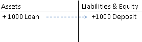
We must recognize, as Minsky did, that banking is a profit-seeking business that is based on very high leverage ratios. Further, banks serve an important public purpose and thus are rewarded with access to the lender of last resort and to government guarantees. What this means is that as soon as capital ratios decline toward some minimum (zero in the case of an institution subject only to market discipline, or some positive number set by government supervisors as the point at which they take-over the institution), management will “bet the bank” by seeking the maximum, risky, return permitted by supervisors. In any event, there is always an incentive to increase leverage ratios to improve return on equity. Given that banks can finance their positions in earning assets by issuing government-guaranteed liabilities, at a capital ratio of 5% for every $100 they gamble, only $5 is their own and $95 is the government’s. In the worst case, they lose $5 of their own money; but if their gamble wins, they keep all the profit. Imagine if you walked into a casino and the government gave you $95 to gamble with, for every $5 of your own—and you get to keep all the winnings. What would you do? Gamble! If subjected only to market forces, profit-seeking behavior would be subject to many, and frequently spectacular, bank failures. The odds are even more in their favor if government adopts a “too big to fail” strategy—although exactly how government chooses to rescue institutions will determine the value of that “put” to the bank’s owners.

Note that while the Basle agreements were supposed to increase capital requirements, the ratios were never high enough to make a real difference, and the insitutions were allowed to assess the riskiness of their assets for the purposes of calculating risk-adjusted capital ratios. If anything, the Basle agreements contributed to the financial fragility that resulted in the global collapse of the financial system. Effective capital requirement would have to be very much higher, and if they are risk-adjusted, the risk assessment must be done at arms-length by neutral parties. I think that if we are not going to closely regulate financial institutions, capital requirements need to be very high—maybe 100%. We used to have “double indemnity”: owners of banks were personally liable for twice as much as the bank lost. That, plus prison terms, would perhaps give the proper incentives.

6- Do you think we need a strict regulation of the financialisation of commodity markets (particularly oil) as Sarkozy, Gordon and the US regulator claimed, or this is a window for non-commercial investors that came to stay?

As implied above, any institution that has explicit or implicit government guarantees—either through deposit insurance or “too big to fail” policy absolutely must be closely regulated.

7- Do you think the sovereign wealth funds and the Asian banks from high liquidity countries (now the 3 top banks in capitalization are Chinese) will be dragged down by the crisis or they can lead a new financial capital wave?

No, I do not think they will lead a new financial wave over the next few years. There is little doubt that the Chinese economy will continue to become important and in the near future will displace the US economy as the largest in the world. It is certainly possible that its currency will eventually displace the dollar as the global reserve currency–but I think that is a long way off. I do not think it is even a role that the Chinese authorities would want right now. Finally, China uses markets where they work, but happily intervenes where markets do not fulfill the public purpose as defined by the government. Hence, I do not believe they would let their own domestic money managers “run wild” in the same way that the more market-oriented (neo-liberal) governments have done. After all, the Premier of China has no fear of being labeled a “socialist”–unlike President Obama!

Obviously, global financial losses are already huge, and will grow much larger over the coming years. Only the debt of sovereign nations is safe. Again, I hope, and expect, that we are seeing an end to this phase of finance capitalism. It will, of course, rise again—eventually. But with proper responses by governments around the world, we might be able to develop the conditions necessary for another “golden age”. Still, as Minsky said, stability is destabilizing so a golden age will allow finance capital to return. There is no “final solution” to the fundamental flaws of capitalism: an arbitrary and excessively unequal distribution of income and wealth, an inability to generate full employment, and a propensity toward financial instability.

Another Take on the Financial Balances

By Eric Tymoigne

First, regarding the identity itself, for a domestic economy we have, in terms of economic flows:

GFB + PDFB + RWFB ≡ 0

With PDFB the private domestic financial balance, RWFB the financial balance of the Rest of the World, and GFB the government financial balance. This identity holds all the time, in any domestic economy (in a world economy RWFB disappears). For economic analysis, it is insightful to arrange this identity differently in function of the type of monetary regime.
In a country that is monetarily sovereign the federal government has full financial flexibility. By monetary sovereignty, one means that there is a stable and operative federal/national government that is the monopoly supplier of the currency used as ultimate means of payment in the domestic economy, and that the domestic currency is not tied to any asset (like gold) or foreign currency. Other posts have already explained the implications of this in terms of federal government finance (taxes and T-bonds do not act as financing sources for federal government spending, the federal government always spends by creating monetary instruments first, etc.) and banking (bank advances create deposits, credit supply is endogenous and is created ex-nihilo (i.e. banks do not need depositors to be able to provide an advance of funds to deficit spending units), higher reserve ratios do not constrain directly the money supply process in a multiplicative way, etc.). All this also has implications in terms of accounting and in terms of modeling.

First, in terms of accounting identity, in a monetarily sovereign country, the government financial balance (GFB), through the federal government financial balance, is the ultimate means to accommodate the changes in holdings of the domestic currency by other sectors (private domestic sector and the Rest of the World). This means that, for a monetarily sovereign country, the most insightful way to arrange the national accounting identity is:

-GFB ≡ PDFB + RWFB

or

-GFB ≡ NGFB

Where NGFB is the non-government financial balance (the sum of the financial balance of the private domestic sector and the Rest of the World). This way of arranging the identity shows well that the government sector (through its federal branch) is the ultimate provider/holder of domestic currency: government fiscal deficit (surplus) is always equal to non-government financial surplus (deficit). The graph below shows the identity for the US.

Fiscal balances for the United State (billions of dollars)

Source: BEA (Table 5.1).
Note: Statistical discrepancy was distributed evenly among the three sectors (Private Domestic, Rest of the World, and Government).

Any net injection of dollars (i.e. financial deficit) by any sector must be accumulated somewhere else (i.e. financial surplus). As the monopoly supplier of ultimate domestic means of payment, usually the US government sector is the net injector of dollars, while the private domestic sector and the Rest of the World usually accumulate the dollars injected. For a while, like from 1997 to 2007 in the US, the private domestic sector and the Rest of the World may transfer the domestic currency among each other while the government runs a surplus; however, this cannot last because ultimately one of them (private sector or Rest of the World) will run out of domestic currency and/or will have to become highly indebted in domestic currency leading ultimately to a Ponzi process that collapses. Only the federal government has a perfect creditworthiness and can always meet its financial obligations denominated in the domestic currency (that is why US Treasury bonds are not rated, default rate is zero).

In addition, one may note that the Rest of the World and the private sector cannot accumulate any domestic currency unless the government sector injects them in sufficient quantity in the first place. Stated alternatively, the Rest of the World (e.g., the Chinese) does not help to finance the deficit of the federal government (US federal government). On the contrary, the federal government deficit allows the Rest of the World to accumulate dollars. This pressure to generate a deficit is all the more strong on the dollar that it is the reserve currency of the world, so there is a net demand for the dollar from the Rest of the World.

This also works the other way around, i.e. if the Rest of the World disaccumulates the domestic currency the government must be the ultimate acquirer of this domestic currency and so must run a surplus if the private domestic sector does not accumulate it in a large enough quantity.
Once it acquires the domestic currency, the government may destroy them (federal government has huge shredders or they are deleted from the computer memory), or store them into a safe/computer for later use (especially true for state and local governments). Destruction of bank notes occurs usually because they are in bad shape. Hundreds of millions of dollars worth of bank notes are destroyed every month at the Fed banks in the US; then they are used as compost (during my last tour of the San Francisco Fed last March, I was told that about $56 million worth of bank notes are destroyed every day at the SF Fed, and then are spread on the fields of California). If you go visit a fed bank this will be the main attraction.

Besides the poor condition of some bank notes, the destruction of dollars by the federal government may also occur for other reason, e.g., because there is a lack of storage capacity (safe is too small, computer memory is too small). One central point is that the dollars that are accumulated by the federal government do not increase its financing capacity because the federal government created those dollars in the first place. It chooses not to destroy them all because it takes time and it is costly to destroy and to make monetary instruments, and because it has the storage capacity.

For the moment, we stayed at the level of the identity, which basically tracks where the domestic currency comes from and where it goes. Every dollar comes from somewhere and must go somewhere. There is no dollar floating around that is not held by a sector. No desire/behavioral equation were included in the analysis above. However, even that basic identity provides us a powerful insight. Indeed, it shows us that it is impossible for all sectors to be in surplus; at least one of them must deficit spend and usually it is the government sector because of its monetary sovereignty. The reverse is also true, i.e. not all sectors can be in deficit at the same time; at least one of them must be in surplus (usually the private domestic sector). As Randy noted in a previous post, this is probably not understood well; even the Wall Street Journal did not make the connection in early the 2000s between the federal government surplus and the households’ negative saving. It is often assumed that if they wish, all sectors could be in surplus; one just needs to work hard enough at it (note that this is one of the promises that is always made during presidential campaigns: “we should save more, reduce our trade deficit and reach a fiscal surplus”). Economic reality does not work that way.

In terms of the model (where one includes desires and so behavioral aspects as well as an explanation of the adjustment mechanisms to those desires in relation to the state of the economy), for the analysis of a monetarily sovereign country, I would rather put the desired financial balance of the Rest of the World with the desired private domestic financial balance and call the sum the desired financial balance of the non-government sector (NGFBd). The model does not deal with stocks at all and their relation to flows (IS-LM did try but failed to do it correctly; read Hicks’s own account in his JPKE article “IS-LM: An explanation”); however, the financial-balance model is a good place to start in Econ 101. If students can understand the model, the identity and how they relate to each other, it would be a HUGE step forward in terms of removing this counterproductive phobia of government fiscal deficits (then one would have to learn about government finance and the monetary creation process, which, like many other things, are all taught backward in textbooks).

If the Rest of the World has too many dollars relative to its taste it and cannot bring them back into the domestic economy, by buying enough goods and services or financial assets from the private domestic and government sectors, the currency depreciates and/or long-term interest rate falls. This boosts exports and reduces imports. This may also promote investment and consumption if the state of expectations is stable.

If the non-government sector desires to save more, then, unless the government sector increases its spending propensity or reduces tax rates, the economy will enter a slump; possibly a debt-deflation process if debt levels are far too high. All this was done nicely in previous posts.
Before, during, and after the adjustment processes (variation of flows, levels and prices) the identity holds and the actual financial balance always sum to zero. The sum of GFBd and NFGBd will be different from zero except when the adjustment is completed, i.e. when actual and desired balances are equal (“at equilibrium” if you want to call it that way, even though markets may not be cleared).

Another Embarrassing Blunder by Chairman Bernanke

By Felipe Rezende

The Fed chairman Ben Bernanke in his recent op-ed piece argued that “given the current economic conditions, banks have generally held their reserves as balances at the Fed.” This is not surprising since, in uncertain times, banks’ liquidity preference rise sharply which reflects on their desire to increase their holdings of liquid assets, such as reserve balances, on their balance sheets.

However, Bernanke pointed out that “as the economy recovers, banks should find more opportunities to lend out their reserves.” The reasoning behind this argument is the so-called multiple deposit creation in which the simple deposit multiplier relates an increase in reserves to an increase in deposits (Bill Mitchell explains it in more details here and here). This is a misconception about banking lending. It presupposes that given an increase in reserve balances (RBs) and excess reserves, assuming that banks do not want hold any excess reserves (ERs), the multiple increase in deposits generated from an increase in the banking system’s reserves can be calculated by the so-called simple deposit multiplier m = 1/rrr, where rrr is the reserve requirement ratio (let’s say 10%). It tells us how much the money supply (M) changes for a given change in the monetary base (B) i.e. M=mB. In this case, the causality runs from the right-hand side of the equation to the left-hand side. The central bank, through open market operations, increases reserve balances leading to an increase in excess reserves in which banks can benefit by extending new loans: ↑RBs → ↑ER → ↑Loans and ↑Deposits.
However, in the real world, money is endogenously created. Banks do not passively await funds to issue loans. Banks extend loans to creditworthy borrowers to meet the needs of trade. In this process, loans create deposits and deposits create reserves. We can illustrate this using T-account as follows:

The bank makes a new loan (+1000) and at the same time the borrower’s account is credited with a deposit of an equivalent amount of the loan. Thus, “the increase in the money supply is a consequence of increased loan expenditure, not the cause of it.” (Kaldor and Trevithick, 1981: 5)
In order to meet reserve requirements, banks can obtain reserves in secondary markets or they can borrow from Fed via the discount window.

As noted by Kaldor (1985), Minsky (1975), Goodhart (1984), Moore (1988), Wray (1990), Lavoie (1984) to name a few, money is endogenously created. The supply of money responds to changes in the demand for money. Loans create deposits and deposits create reserves as explained here and here. It turns the deposit multiplier on its head. Goodhart (1994) observed that “[a]lmost all those who have worked in a [central bank] believe that [deposit multiplier] view is totally mistaken; in particular, it ignores the implications of several of the crucial institutional features of a modern commercial banking system….’ (Goodhart, 1994:1424).
As Fulwiller put it, “deposit outflows, if they exceed the bank’s RBs, result in overdrafts. Banks clear this via lowest cost available in money markets or from the Fed.” In this case, let us assume that the bank issues some other liability, such as CDs, in order to obtain the 1000 reserves needed for clearing its overdraft at the Fed.

It reverses the orthodox story of the deposit multiplier (M=mB). Banks are accepting the liability of the borrower and they are creating their own liability, which is the demand deposit. In this process, banks create money by issuing its own liability, which is counted as a component of the money supply. Banks do not wait for the appropriate amount of liquid resources to exist to provide new loans to the public. Instead, as Lavoie (1984) noted ‘money is created as a by-product of the loans provided by the banking system’. Wray (1990) puts it best:
“From the bank’s point of view, money demand is indicated by the willingness of the firm to issue an IOU, and money supply is determined by the willingness of the bank to hold an IOU and issue its own liabilities to finance the purchase of the firm’s IOU…the money supply increases only because two parties willingly enter into commitments.” (Wray 1990 P.74)

As showed above, when banks, overall, are in need of more high-powered money (HPM), they can increase their borrowings with the central bank at the discount rate. Reserve requirements (RRs) cannot be used to control the money supply. In fact, RRs increase the cost of the loans granted by banks. As Wray pointed out “in order to hit the overnight rate target, the central bank must accommodate the demand for reserves—draining the excess or supplying reserves when the system is short. Thus, the supply of reserves is best characterized as horizontal, at the central bank’s target rate.” The central bank cannot control even HPM!The latter is provided through government spending (or Fed lending). The central bank can only modify its discount rate or its rate of intervention on the open market.

Bernanke is concerned that the sharp increase in reserve balances “would produce faster growth in broad money (for example, M1 or M2) and easier credit conditions, which could ultimately result in inflationary pressures.” He is considering the money-price relationship given by the old-fashioned basic quantity theory of money relating prices to the quantity of money based on the equation of exchange (The idea that money is related to price levels and inflation it is not a new idea at all, you can find that, for example, in Hume and other classical economists):

M*V = PQ, where M stands for the money supply (which in the neoclassical model is taken as given, i.e. exogenously determined by monetary policy changes in M), Q is the level of output predetermined at its full employment value by the production function and the operation of a competitive labor market; P is the overall price level and V is the average number of times each dollar is used in transactions during the period. Causality runs from the left-hand side to the right-hand side (nominal output)

According to the monetarist view, under given assumptions, changes in M cause changes in P, i.e. the rate of growth of the money supply (such as M1 and M2) determines the rate of change of the price level. Hence, to avoid high inflations monetary policy should pursue a stable low growth rate in the money supply. The Fed, under Paul Volcker, adopted money targets in October 1979. This resulted in extremely high interest rates, the fed-funds rate was above 20%, the US had double digit unemployment and suffered a deep recession. In addition, the Fed did not hit its money targets. The recession was extremely severe and in 1982 Volker announced that they were abandoning the monetarist experiment. The rate of money growth exploded to as high as 16% p.y, over 5 times what Friedman had recommended, and inflation actually fell (see figure below).

Source: Benjamin Friedman, 1988 :55

The Collapse of the Money-Income and Money-Price Relationships

A closer look at the 1980s and 1990s help us understand the relationship between monetary aggregates such as M1 and M2 and inflation. This is a relationship that did not hold up either in the 1980s nor in the 1990s. As Benjamin Friedman (1988) observed “[a]nyone who had relied on prior credit-based relationships to predict the behavior of income or prices during this period would have made forecasts just as incorrect as those derived from money-based relationships.” (Benjamin Friedman, 1988:63)

Despite the collapse of the relationship between monetary aggregates and inflation Bernanke still believes that “we must either eliminate these large reserve balances or, if they remain, neutralize any potential undesired effects on the economy.” He noted that “we will need to tighten monetary policy to prevent the emergence of an inflation problem down the road” However, is inflation always and everywhere a monetary phenomenon? The answer is no. The picture below plots the credit-to-GNP ratio. Note that even “the movement of credit during the post-1982 period bore no more relation to income or prices than did that of any of the monetary aggregates.” (Benjamin Friedman, 1988:63, emphasis added)

What about the other monetary aggregates? Benjamin Friedman (1988) pointed out that “[t]he breakdown of long-standing relationships to income and prices has not been confined to the M1 money measure. Neither M2 nor M3, nor the monetary base, nor the total debt of domestic nonfinancial borrowers has displayed a consistent relation- ship to nominal income growth or to inflation during this period.” (ibid, p.62)

Even Mankiw admitted that “[t]he standard deviation of M2 growth was not unusually low during the 1990s, and the standard deviation of M1 growth was the highest of the past four decades. In other words, while the nation was enjoying macroeconomic tranquility, the money supply was exhibiting high volatility. The data give no support for the monetarist view that stability in the monetary aggregates is a prerequisite for economic stability.” Mankiw, 2001: 33)

He concluded that “[i]n February 1993, Fed chairman Alan Greenspan announced that the Fed would pay less attention to the monetary aggregates than it had in the past. The aggregates, he said, ‘do not appear to be giving reliable indications of economic developments and price pressures’… [during the 1990s] increased stability in monetary aggregates played no role in the improved macroeconomic performance of this era.” (Mankiw 2001, 34)

A recent study conducted by the FRBSF also concluded that “there is no predictive power to monetary aggregates when forecasting inflation.” What about the Japanese experience? As the figure below shows, the monetary base exploded but prices actually fell!

Source: Krugman

What about the US in the 1930s? The same pattern happened, HPM rose sharply and prices were stable!

Source: Krugman

Chairman Bernanke should learn the basic lesson that money is endogenously created. Money comes into the economy endogenously to meet the needs of trade. Most of the money is privately created in private debt contracts. As production and economic activity expand, money expands. The privately created money is used to transfer purchasing power from the future to the present; buy now, pay latter. It allows people to spend beyond what they could spend out of their income or assets they already have. Money is destroyed when debts are repaid.
Consumer price inflation pressures can be caused by struggles over the distribution of income, increasing costs such as labor costs and raw material costs, increasing profit mark-ups, market power, price indexation, imported inflation and so on. As explained above, monetary aggregates are not useful guides for monetary policy.

Another Great Depression?

By Felipe Rezende

In a previous post, I explained that automatic stabilizers- i.e. the fact that the federal government’s budget moves counter-cyclically and in an automatic fashion – imparts a great stabilizing force to aggregate demand.
However, the picture below shows that, during the Great Depression the government sector was too small relatively to the rest of the economy.

Source: Tymoigne, 2008: 12

The implementation of New Deal policies created automatic stabilizers which work by putting a floor under aggregate demand, preventing a deflationary spiral, but they also put ceilings in place, as rapid economic growth translates into rising tax revenues which destroy income and temper the expansion.
Nowadays, the size of the government and the impact of large automatic stabilizers explain why we can have a deep recession but another Great Depression is unlikely.
But how do automatic stabilizers work? What happens over the cycle? Hyman Minsky sheds light on these issues.

Minsky’s financial instability hypothesis can be described as follows. Let us consider that the whole U.S. economy is in a hedge position, i.e. that cash inflows are greater than outflows for every period, so that debt/payment commitments can be fulfilled while safety margin are kept at some positive level, for instance 20%. As firms and households become more optimistic about future earnings, and as their expectations get validated by economy growth, they change their behavior and reduce their margins of safety, let’s say now to 10%.

As the economy booms, and future earnings turn out to be more than expected, firms and households revise their expectations upwards, they begin to believe they were too pessimistic in the past and, therefore, reduce their cushions of safety, and start to take on more and more riskier projects. They have voluntarily moved into a position Minsky called speculative. A speculative position is one in which cash inflows are enough to meet interest payments, i.e. as they cannot repay the principal they need to refinance the outstanding debt. Borrowers start to discount risk and lenders, now more optimistic about prospective future earnings and profits, increase their willingness to lend.

It is now important to introduce how the level of investment is determined according to Minsky’s framework. Firms invest if the demand price of capital exceeds the supply price of current output. “The quantity of investment goods purchased (OId) is determined where PId = PIs” (Tymoigne and Wray 2008, p.9)

The demand price, Pk, is the price that firms are willing to pay for the capital asset. The demand price depends upon the cash flows that ownership is expected to yield and the liquidity of the asset. The curve is horizontal up to the point where firms only commit their internal funds. However, once firms rely on external financing then the subjective borrower’s risk comes into play. This risk is incurred by firms as they may not be able to service their debt. Thus, the price that firms are willing to pay for capital assets decline as the amount they have to borrow to finance it increases.

The supply price, Pi, is the price that firms actually have to pay for the capital good. Firms can use their internal funds up to Oif , and only up to this point, the supply price equals costs + markup. When firms have to borrow to buy capital goods, the supply price of investment is raised by the interest payments on the loan. The curve slopes up after the point Oif because of the lender’s risk. The lender’s risk is the risk the firm will not repay the loan. The more the individual firm borrows, the greater the lender’s risk associated and the higher the interest rate charged on the loan.

When lenders and borrowers become more optimistic about future earnings and profits, they start to discount risks. Firms take on riskier projects and financial institutions riskier loans. Thus, the belief is now that future income will be enough to cover debt commitments. They are in a speculative position.

If there is a change in the economic environment firms’ financial positions may be adversely impacted. Let’s consider the following situation where the economy accelerates and inflation becomes a concern to the monetary authority. The turning point would happen when the Fed decides to increase the overnight interest rate. If the interest rate specified on contracts is allowed to fluctuate, firms incur in higher financial costs to service the loan. At the new circumstance, firms can either abandon the project, as it is no longer profitable at higher interest rates, or they can borrow, from willing financial institutions, the funds they need to meet the interest payments on the previous loans. In other words, if interest rates are increased to such a point where firms’ income inflows are no longer sufficient to meet the firms’ outflows, they have involuntarily moved into a new financial position that Minksy called Ponzi. In a Ponzi scheme, firms have to capitalize interest. If financial institutions become worried about the future performance of the economy as a whole or the firm in particular, and decide to no longer extend those Ponzi loans, then firms are no longer capable of meeting their financial commitments and may default on their loans. This situation can be compounded as firms decide to sell their assets at fire sale prices in order to meet their obligations, setting in a Fisher-type debt deflation process which triggers a domino effect on the economy.

Another situation we could consider as a turning point is one in which firms’ expectations about future earnings/profits is not fulfilled. In such an environment, firms will revise their expectations downwards and cut investment. As we know, this will have a multiplier effect in the economy. As income is reduced, so is consumption. Firms cut back production and investment, which depresses incomes further. The economic activity spirals down squeezing incomes even more. As firms’ income inflows were significantly reduced, firms may get to a point where they can no longer meet their liability commitments. Once again, a debt-deflation process may be set in place by the new economic environment when firms decide to sell their assets at fire sale prices trying to meet their obligations.

Now, we may ask ourselves: what is the role of automatic stabilizers in this process?
The answer becomes even clearer. With big government automatic stabilizers are large enough to offset the swings in private spending. As explained in a previous post, when the economy goes into recession, unemployment rises which means that income transfers such as unemployment compensation and welfare are automatically increased.

According to Minsky, there are 3 major effects derived from automatic stabilizers: the income and employment effect, the cash flow effect, and the portfolio effect. Let me briefly explain each one:

The income effect is the traditional Keynesian multiplier. As the economy slows down, the government deficit increases as there is an automatic increase in spending and a reduction of the amount of taxes collected. As noted in previous posts (here and here), a sovereign government spends by crediting bank accounts which means that the banking system, all else equal, now has excess reserves (ERs). The ERs put a downward pressure on the fed funds rate. If the Fed is to hit its overnight nominal interest rate target, it has to intervene and conduct open market sales (OMS) to drain the ERs. As the Fed provides an interest bearing alternative – such as government securities – this is adds to the private sector’s income.
Therefore, transfer payments and interest payments automatically increase when the economy is moving into a recession.

The other one is the cash flow effect. The idea is that government deficits maintain the flow of profits. Following Kalecki (1972) and national accounting identities, in the simplest version, aggregate profits equal investment plus the government’s deficit, Π = Invest. + Gov. Deficit. In the expanded model, gross profits, after corporate tax, equals investment plus government fiscal deficit plus consumption out of profits plus net exports less saving out of wages, i.e. Π = Invest. + Gov. Deficit + CC + NX– SW. This means that government deficits add to profits (private wealth). The flow of profits prevents the collapse of expectations and the deterioration of private sector’s balance sheet.

Finally, the portfolio effect is generated by the increase in the sale of government bonds as a consequence of the (mostly automatic) increased government deficit (as I have just explained). These bonds are safe assets and their holdings on private sector’s balance sheets help to keep expectations from collapsing below a certain level.

The Big Bank (the Fed) act as a lender of last resort, it can prevent or minimize the fall in asset prices. In other words, the Fed can always put a floor to asset prices. This can be done in many ways, such as by calling up banks and say that they need to lend to investors who want to buy assets. The Fed can also decide to buy a wide range of private assets to smooth market transactions. If the Fed decides to buy a wide range of assets to provide liquidity to markets it smoothes liquidity concerns of market participants. It can also regulate markets and discourage bad loans such as subprime real state booms in some regions so that banks will not provide those loans. However, ceilings should also be put in place such as supervision and regulation, as has been emphasized by William K. Black.

In the current recession, the forecast is that the personal saving rate will reach something like 10% in 2009 and that it could jump to 14-16% by 2010. To meet the private sector rising saving desire the government should implement another stimulus package (in the context of the Krugman’s cross described here, this would be equivalent to a shift of the government sector balance -GSB- curve to the right) thus preventing a deflationary spiral and further declines of income due to rising private sector saving desire. At the same time, it becomes important to adopt policies that make the curve steeper by enhancing the role of automatic stabilizers. One possibility is an employer of last resort program in which the federal government provides a job to everyone willing and able to work at a given nominal wage. As argued in previous posts(here and here) such program would reduce both unemployment and poverty and minimize declines in the economic activity by enhancing the ceilings and floors of the system.

A Third Stimulus Package and Job Creation

Our own L. Randall Wray and Lawrence Mishel say that additional stimulus is needed to create jobs immediately.

http://www.reuters.com/resources/flash/include_video.swf?edition=US&videoId=108026

Read more here, here, here, and here.

Krugman’s New Cross Confirms It: Job Guarantee Policies Are Needed as Macroeconomic Stabilizers

By Daniel Negreiros ConceiçãoKrugman’s new explanation of business cycles in the form of a GSFB-PSFB (government sector financial balances – private sector financial balances) model (see his post entry here) has invoked a sort of call-to-arms by some dedicated Keynesian economists. Though those of us who have acquired the habit of looking at both sides of every nominal flow in the economy may see less novelty in Krugman’s new framework, the cross itself is still a very nice tool for presenting our arguments. And, if Krugman’s cross actually succeeds in replacing the unfortunate IS-LM interpretation of Keynes’ General Theory, it will have moved the New Keynesian approach in a constructive new direction.

I will not rehash the details of the Krugman cross in this post, since other bloggers have already explained the cross and some of its implications (see, e.g., Rob Parenteau’s, Scott Fullwiler’s, and Bill Mitchell’s). Instead, I want to draw out a particular (and potentially revolutionary) implication of the model.
I believe that what Krugman was able to finally see, with the help of his cross, is nothing but the restatement of Keynes’s old paradox of thrift for a closed economy with a government sector able to run a deficit (though one can also represent the original paradox of thrift taught in intermediate macroeconomics if the GSFB – government sector financial balances – curve coincides with the horizontal zero deficit/surplus line, i.e. if governments run a balanced budget). Much like the simple exposition of the paradox of thrift for a closed economy without a government sector where aggregate savings are unavoidably equal to the size of aggregate investments, in an economy with a government sector the value of the private sector surplus is unavoidably determined by the government deficit. This means that when the desired level of private sector surplus rises as a share of each level of GDP, the tautological stubbornness of the accounting identity forces the adjustment to take place in one of two ways (or a combination of both). Either:(1) The government deficit rises so that the private sector is able to achieve its new desired level of surplus at the current level of GDP

or

(2) GDP must fall until the GS (government sector) deficit reaches the new desired level of PS (private sector) surplus as a share of GDP

This is the exact equivalent to what Keynes argued with regard to an increase in the propensity to save. When people decide that they want to save more as a share of their incomes (or alternatively, when capitalists decide to increase the mark up over wage costs), for a given level of aggregate investment, aggregate incomes must fall so that the same aggregate savings becomes a greater share of the reduced aggregate income. As Rob Parenteau argued, “If Paul [Krugman] recalls his reading of Keynes’ General Theory (and he is to be applauded for being one of the few New Keynesians to actually read Keynes in the original), this is one of the reasons Keynes argues incomes adjust to close gaps between intended investment and planned saving.”

It is time to play a little with the shapes of the curves. Here I believe that Krugman’s analysis is especially useful for explaining policy prescriptions advanced by Post Keynesian economists. First of all, in the GSFB-PSFB model I see none of the interdependency problems and stock/flow inconsistencies that exist in the IS-LM model (so far…). As many of the bloggers (Felipe Rezende here) have demonstrated, under the current set of economic policies in the US, GS deficits tend to rise substantially when GDP falls also substantially. In Krugman’s framework this is represented as a relatively steep GSFB curve. The steeper the curve, the faster the deficit increases for a given reduction of GDP bellow a given threshold (given by the level of GDP where the GSFB curve intercepts the zero surplus/deficit horizontal axis). However, it is also true that the same government who responds promptly to a fall in GDP by raising its deficit significantly also responds aggressively to an increase in GDP above the threshold by raising its surplus since the curve is equally steep going down below the intercept as it is going up above it. Maybe we should represent the curve as having different steepness below and above the threshold, but this is less important as it depends on more sophisticated assumptions about government policies. While Prof. Krugman makes the interesting and convincing argument that the fact that today’s GSFB curve is much steeper than that of the early 1930s (meaning that GS deficits in the 30s did not rise significantly despite a great reduction in aggregate incomes) has kept us from experiencing another Great Depression, we have just begun to experiment with the shapes of the curve.

First of all, let us look at extreme situations:

(1) In the absence of government deficits or surpluses in the economy (i.e. if governments were blindly committed to having balanced budgets), the horizontal GSFB curve would coincide with the zero deficit/surplus line and changes in desired PS surplus out of savings would necessarily lead to aggregate income adjustments so that new equilibrium would be reached at the new intercept where PS surplus was zero. Income fluctuations would be the most violent under these conditions since changes in spending preferences by the private sector would lead to full income adjustments. Note that any horizontal GSFB curve would produce such effect. In other words, macroeconomic instability is the result not of the unwillingness of governments to run a deficit (indeed a horizontal GSFB curve above the horizontal axis could represent any size of GDP independent GS deficits), but of governments not adjusting the size of their deficits to changes in spending propensities out of given incomes.

(2) What if governments decided to determine the level of GDP for the economy (hopefully at full employment)? Then governments could accommodate any change in the level of desired PS surplus by raising and reducing its deficit accordingly so that GDP never needed to adjust. This would be represented by a vertical (or, more realistically, almost vertical if some GDP adjustments still took place) GSFB curve at full employment GDP. These are the kind of policies we should be looking for as automatic stabilizers: policies that make the GDFB as close to vertical as possible at full employment GDP. The most effective way to achieve it: an employer of last resort policy where changes in desired PS surplus at full employment GDP that lead to falling aggregate expenditures and employment in the private sector would be largely compensated by increases in government transfers to the newly hired workers in the form of wages. Even though it is not necessarily the case that the deficit brought about by such policy will be exactly equal to the new desired PS surplus at full employment GDP so that the GSFB is completely vertical, in addition to other stabilizers such policy will significantly raise the steepness of the curve.

Krugman has hit on something of great importance. I hope others will think through the implications of his approach and not allow the momentum to wane.

Washington Finally Proposes Real Help to Deal with Foreclosures

By L. Randall Wray

The Washington Post reported on Friday that Washington is finally considering meaningful steps to deal with the on-going foreclosure crisis. The article reports:

“A top Treasury Department official told a Senate panel yesterday that the government is considering a proposal to allow homeowners to stay in their home as renters after a foreclosure.”

The administration appears to be conceding that all of its proposals to date have been complete flops. The report goes on:

“Under the federal program known as Making Home Affordable, lenders are paid to lower borrowers’ mortgage payments. About 160,000 loans have been modified into lower-cost loans so far. The administration has said the federal effort has already been more successful than previous programs.”


That program was designed by the lenders, who wanted yet another government hand-out. But it was doomed to fail because mortgages that have been packaged into complex securities cannot be modified easily. If, instead, the government had directed aid to homeowners from the very beginning, it could have slowed the downward spiral of real estate markets. Reports yesterday put the number of foreclosures this year at another 2 million, with similar projections for next year. What is needed now is relief for the millions of families who have lost, or will soon lose, their homes.

Allowing families to stay on as renters after a foreclosure is a step in the right direction. However, the government should go further by following the plan put forward by Warren Mosler, as I summarized previously:

When banks begin to foreclose, the government would step in to purchase the property at the lower of market price or outstanding mortgage balance. Establishing market price in a glut is not simple, but it is not impossible. Mosler proposes that the federal government would rent homes back to the dispossessed owners (Dean Baker has a similar plan) for a specified period (perhaps two years) at fair market rent. At the end of that period, the government would sell the home, with the occupant having the right of first refusal to buy it. Reducing evictions by offering a rental alternative will help reduce the pain of foreclosure. It might also allow the process to speed up (with smaller losses for banks) since many families would choose to stay-on as renters, with the possibility that they could later buy their homes at more reasonable prices.

The Sector Financial Balances Model of Aggregate Demand

By Scott Fullwiler

Paul Krugman’s recent post indicates that perhaps those of us taking a stock-flow consistent approach to macroeconomics may be making some headway. My fellow blogger, Rob Parenteau, and another friend, Bill Mitchellboth describe many of the details of this approach and how they fit the graph posted by Krugman. Rob is correct to suggest this would be a much better framework for understanding macroeconomics than the traditional IS-LM model, which was highly flawed to begin. My purpose here is to build on both of these posts and demonstrate a few uses of the model (thus, those not familiar with this framework should read Rob’s and/or Bill’s posts first, probably).To begin, consider the graph in Krugman’s post below:

Continue reading

Employing Krugman’s Cross: Farewell, Mr. Hicks?

By Robert Parenteau

Paul Krugman’s July 15th blog post diagramming financial balances makes some important steps in revealing the analytical power of the financial balance approach to macroeconomics – something once understood by J.M Keynes and early Keynesians like Nicholas Kaldor, Abba Lerner, and Joan Robinson, but long since lost in the headlong rush over the past three decades of mainstream macroeconomics to become a special branch of microeconomics, which itself appears to have become a special branch of applied calculus in some sort of rather twisted physics envy. I suspect reading Minsky has helped Paul immeasurably in seeing these relationships, and I would urge him and others to go find some of Wynne Godley’s contributions (many of which are available online at the Levy Economics Institute) to a stock/flow coherent macroeconomics, and it may all become that much clearer.

The diagram Paul presented at first (reproduced below) threw me for a loop, but I believe I now see what he was doing, as the labeling did not initially make it clear, and perhaps by walking through Paul’s diagram, others can avoid my initial confusion.


The upward sloping line should be labeled the private sector financial balance (PSFB), and the downward sloping line should be labeled the government financial balance (GFB). Only the part of the PSFB schedule above the horizontal axis is in surplus, if this horizontal GDP axis crosses the vertical sectoral financial balance axis at zero. Similarly, only that part of the GFB schedule above the horizontal axis is in deficit. I believe Paul has defined the vertical axis such that the range above zero represents a rising PSFB, and at the same time, a falling GFB of the same absolute amount, but of opposite sign. Then the area below zero is a falling PSFB and a rising GFB. Above zero represents a private sector financial surplus and a government deficit, while below zero represents a private sector deficit and a government surplus.

Confusing at first, but this follows because Paul has simplified the analysis to two sectors, and sectoral financial balances must balance ex post for any accounting period. The range above zero representing a private sector surplus must also represent a government deficit (GFB must be of equal magnitude but opposite sign to the PSFB). This would seem consistent with Paul’s GFB schedule falling below zero as GDP increases, since a falling fiscal deficit would eventually give way to an increasing fiscal surplus as income increases if automatic stabilizers work as we believe they do (see previous post here). Similarly, the rising PSFB schedule is consistent with traditional Keynesian stability conditions, with saving increasing faster in income than investment does, although we should all keep in mind, as Minsky emphasized, that explosive growth dynamics (Minsky’s upward instability) can arise in economic expansions characterized by euphoric asset pricing. Hence, the last two US business cycle expansions have been characterized by a falling PSFB (that is, deficit spending by the household and business sectors combined), not a PSFB rising as income rises, but that can be accommodated in less simplified versions of Krugman’s cross.

Another way to see why this interpretation of the diagram must be correct is that when the PSFB schedule shifts up and to the left, representing a higher desired net private saving at each level of income, the new point of intersection with the GFB schedule would, for example represent a new short run equilibrium point where say a $250b net private saving position is met by a $250b fiscal deficit. Again, sectoral financial balance must balance ex post (as explained in prevoius posts here and here). If one sector is running a net saving or surplus position, the other sector must be dissaving or deficit spending. That is the tyranny of double entry book keeping – not high Keynesian theory.

If I now have the orientation of the diagram straight in my head (and this is the only way I can see that it makes sense), those who believe in fiscal rectitude may wish to notice two aspects of the world we live in. If you view a balanced fiscal budget as the ultimate and over riding goal, you can get there one of two ways from Paul’s second PSFB schedule (the higher line we seem to have shifted to, as asset prices and profitability have collapsed over the past year, thereby forcing lower private investment and driving saving out of private income flows higher).

To arrive at a fiscal balance, you can shift the GFB schedule down and to the left by jamming tax rates higher and lowering the government spending propensities out of tax revenue income until the GFB schedule intersects the PSFB schedule at the point where the PSFB schedule crosses the horizontal axis at the zero financial balance mark. Notice the level of income the economy is then operating at, and all of you who pay dues to the Concord Coalition, please consider whether existing private debt loads could actually be serviced at that lower level, since most private debt contracts are fixed nominal payment commitments. Think post Lehman bankruptcy, on steroids, and you might get a taste of what you are praying for with perpetually balanced fiscal budgets.

The second way to get to a fiscal balance is to encourage the PSFB schedule to shift down and to the right until it intersects the GFB schedule at the point at which it crosses the horizontal axis. That means increasing incentives for the private sector to invest more money at each income level and save less money at each income level. Given the residential housing stock overhang, and the need for households to save out of income flows if they cannot rely on serial asset bubbles to deliver the appropriate nominal net worth at retirement, that means ways must be found to encourage US businesses to pursue a higher reinvestment rate in the US, rather than borrowing money to buy back shares to boost stock prices or reinvesting abroad. Not easy, but not impossible either. Notice also that the second form of adjustment leaves you at a higher equilibrium income level, and the existing private debt to GDP ratio will stabilize, since there will be no additions to the private debt stock, as net private deficit spending is zero at the new income flow level.

Of course, this should all eventually be recast in dynamic terms. For example, income won’t grow unless the GFB is continually shifting up and to the right, or the PSFB is continually shifting down and to the right (or some combination of the two). There is also no obvious endogenous mechanism shifting the PSFB toward a position of full employment income over time, given the position of the GFB. Of course, in theory, policy could be geared such that given reasonable estimates of the likely position of the PSFB schedule, the GFB schedule could be shifted out (or less likely, in) to achieve the level of income associated with full employment. Alternatively, fiscal policy could be structured so the GFB schedule could be perfectly vertical at the full employment level of income, which in many ways is what an employer of last resort (ELR) driven fiscal policy attempts to do.

Finally, for those insistent that public and private debt to income ratios must be held fixed from here to eternity for whatever reason, then starting from Paul’s initial equilibrium, income growth could only be accomplished if the PSFB schedule could be encouraged to shift outward, and the GFB could be shifted in concert such that either the realized financial balances of both sectors were kept at zero, or there was some cycling between the two, such that periods of private sector financial deficits were followed by periods of government sector deficits of similar magnitude and duration.

The trade balance must also be brought back into the story, as a trade surplus is the only way both the GFB and the PSFB can maintain a net saving position at the same time (assuming for whatever reason that was a worthy goal), but at least it is a promising start at representing how sectoral financial balances are related, and it reveals many of the misconceptions that unnecessarily cloud the debate.

If the Krugman Cross does nothing more than provide a stepping stone away from the dead end trap of the Hicks/Harrod/Meade IS/LM diagram, then this is a useful initial contribution. Caught under the spell of IS/LM conventions, Paul and other New Keynesians have spilled far too much ink trying to devise ways of instituting negative real interest rates to get the economies out of a balance sheet driven recession. With policy rates near zero, this analysis has devolved into arguments about how best to increase inflation expectations or actual inflation in order to achieve a sufficiently negative real interest rate. From a practical point of view, the last thing households facing heavy debt servicing loads with falling wage and salary incomes need are rising consumer prices that drain their already reduced discretionary income. Households need higher money incomes, not higher consumer prices, expected or actual, to exit their current difficulties. Real interest rates are diversion from the real problem at hand in a balance sheet recession, which is how to get the economy to a point where money income levels can service most private debts. Krugman’s Cross makes it obvious – shift the GFB schedule in response to shifts in the PSFB schedule.

As always, we must be careful about sliding between the usual ex ante/ex post distinctions, as the income multiplier lies masked behind these interactions, as does the reconciliation of new liability issuance with portfolio preferences, among other balance sheet and asset price considerations that must be brought into play for a coherent stock/flow macroeconomics, of which Hick’s IS/LM approach was a pale shadow that concealed more than it revealed.

For example, the private sector may plan to net save more at any given expected income or GDP level, but unless some other sector net saves less or deficits spends more, private incomes will adjust downward, and the desired private net saving will be thwarted, paradox of thrift style. If Paul recalls his reading of Keynes’ General Theory (and he is to be applauded for being one of the few New Keynesians to actually read Keynes in the original), this is one of the reasons Keynes argues incomes adjust to close gaps between intended investment and planned saving. Interest rates do not equilibrate investment and saving – incomes do, in Keynes’ General Theory. Paul has taken a very large step in this direction with his financial balance diagram, which hopefully he will find more powerful than his IS/LM analytics which he employed in the case of the Japanese balance sheet recession.

Specifically, Paul refers to the need for net private saving being “absorbed” by the public deficit spending. That assumes the net private saving can exist without some other sector deficit spending at the same time, which is impossible. William Vickrey and James Tobin used to make a similar slip, with Vickrey arguing the private saving had to be recycled by public deficit spending (see Vickrey’s otherwise useful piece on 15 fundamental fallacies, linked at CFEPS here.

In Paul’s 2 sector model, unless the public sector spends more money than it takes in as tax receipts, the private sector cannot earn more money than it spends, no matter what its plans or intentions or ex ante designs. Net private saving is created, allowed, or constrained by the size of the public deficit. Net private saving cannot exist as anything more than a hope and a prayer unless some other sector is willing and able to deficit spend. Ex post, in a 2 sector model, as a matter of basic accounting, the net saving of one sector must be equal to the net deficit spending of the other. That is the short run accounting “equilibrium” or reality.

Moving beyond a simple 2 sector model to the world we actually inhabit, it is really as simple as this. The US household sector cannot net save in nominal terms (spend less money than it earns) unless some other sector (or combination of sectors) is willing and able to spend more money than it earns.

It can be the government, the business, or the foreign sector or some mix of the three that net deficit spends – take your choice. But keep in mind, of the three, a government with a sovereign currency (not convertible into fixed quantities of a commodity or another currency on demand) and no debt denominated in foreign currencies is the only one of those three that cannot go bankrupt and cannot default on its debt while continuously deficit spending – unless it chooses to default for some odd political reason.

The sooner we face this fundamental reality of contemporary monetary and economic arrangements, the better. It does not require swearing allegiance to high Keynesian theory – it is simply an accounting reality. Reject it, and you will also have to throw at least seven centuries of double entry book keeping out the window as well.

Since the US economy does appear to have entered a debt deflation spiral for the first time in a lifetime, and it does appears that the spiral has been contained for the moment by a reduction in the trade deficit and a surge in the fiscal deficit, it might be a good time for economists, investors, policy makers, and the general public to once and for all find some clarity on these questions regarding financial balances and the economy. Perhaps Paul’s simple back of the napkin diagram of financial balances takes us one step in that direction.

A note on Automatic Stabilizers

What has so far prevented a deep depression in 2009? The answer, as Paul Krugman explained yesterday, are automatic stabilizers. Indeed, as Hyman Minsky emphasized more than 20 years ago in his book Stabilizing an Unstable Economy (1986), this feature of the federal government’s budget – i.e. the fact that it moves counter-cyclically in an automatic fashion – imparts a great stabilizing force to aggregate demand.

The figure below sheds light on the non-discretionary (i.e. automatic) nature of government deficits. In an economic downturn, tax receipts automatically fall, and government expenditures automatically rise, resulting, automatically, in budget deficits. (net govt saving = right hand scale)

Source: Bureau of Economic Analysis (BEA)

The components of government spending that rise automatically are called ‘transfer payments’, that include unemployment compensation, Medicaid, grants-in-aid to state and local government, etc.
With these forms of payment increasing and tax receipts declining due to falling economic activity, the federal budget moves automatically into deficit.

Source: Bureau of Economic Analysis (BEA)

So far the stimulus package was not what saved the US economy. The budget projections show that 24% of the total cost of the stimulus package will occur in fiscal year 2009 (which means $198 billion) and 47% of it occurring in fiscal year 2010.

“The ARRA is estimated in the budget to cost $825.4 billion over the next 10 years. These costs are split between $600.0 billion in increased outlays and $225.4 billion in reduced receipts. Although the cost of the ARRA is spread over 10 years, the budget projections show 24 percent of the total cost occurring in fiscal year 2009 and 47 percent of the total cost occurring in fiscal year 2010…The budget estimates that receipts will be reduced $77.4 billion in fiscal year 2009 and $152.3 billion in fiscal year 2010 primarily because of the tax provisions of ARRA… The budget estimates that outlays will be increased about $120.2 billion for fiscal year 2009 and $237.8 billion for fiscal year 2010 because of the spending and investment provisions of the ARRA.”

As noted in previous posts (here, here, and here), government deficits, themselves, perform an important stabilizing function, because they allow the private sector to net save. Given that during a recession there is a sharp increase in uncertainty and insecurity, the private sector desires to spend less than its income which translates into a rising personal saving rate. In the current recession, the forecast is that the personal saving rate will reach 10% in 2009 and that jump to 14-16% by 2010. Such large decline in consumption means falling sales, production and further declines in GDP. As noted above, to meet the private sector rising saving desire the government should run bigger deficits to prevent a deflationary spiral.

Source: Jan Hatzius, Goldman Sachs

As Minsky emphasized, the problem, during the Great Depression, was that the government sector was too small relative to the rest of the economy; it couldn’t fill the demand gap and allow the private sector to save as much as it desired. In the absence of large enough automatic stabilizers to offset swings in private spending, GDP contracted to the point where desired net nominal saving equaled actual net nominal saving. Note that in second half of the last century, given the private sector’s desire to have positive net nominal saving, the US government normally ran budget deficits.

As Wray pointed out, “Since WWII we have had the longest depression-free period in the nation’s history. However, we have had nine recessions, each of which was preceded by a reduction of deficits relative to GDP.” This directly results from the impact of large swings in the federal government’s budget.

Automatic stabilizers work by putting a floor under aggregate demand, preventing a deflationary spiral, but they also put ceilings in place, as rapid economic growth translates into rising tax revenues which destroy income and temper the expansion. The impact of large automatic stabilizers explains why we can have a deep recession but not a Great Depression. As Wray noted:

“With one brief exception, the federal government has been in debt every year since 1776. In January 1835, for the first and only time in U.S. history, the public debt was retired, and a budget surplus was maintained for the next two years in order to accumulate what Treasury Secretary Levi Woodbury called “a fund to meet future deficits.” In 1837 the economy collapsed into a deep depression that drove the budget into deficit, and the federal government has been in debt ever since. Since 1776 there have been six periods of substantial budget surpluses and significant reduction of the debt. From 1817 to 1821 the national debt fell by 29 percent; from 1823 to 1836 it was eliminated (Jackson’s efforts); from 1852 to 1857 it fell by 59 percent, from 1867 to 1873 by 27 percent, from 1880 to 1893 by more than 50 percent, and from 1920 to 1930 by about a third. (Thayer 1996) The United States has also experienced six periods of depression. The depressions began in 1819, 1837, 1857, 1873, 1893, and 1929. Every significant reduction of the outstanding debt has been followed by a depression, and every depression has been preceded by significant debt reduction. Further, every budget surplus has been followed, usually sooner rather than later, by renewed deficits. However, correlation—even where perfect—never proves causation. Is there any reason to suspect that government surpluses are harmful?”