The Fed chairman Ben Bernanke in his recent op-ed piece argued that “given the current economic conditions, banks have generally held their reserves as balances at the Fed.” This is not surprising since, in uncertain times, banks’ liquidity preference rise sharply which reflects on their desire to increase their holdings of liquid assets, such as reserve balances, on their balance sheets.
However, Bernanke pointed out that “as the economy recovers, banks should find more opportunities to lend out their reserves.” The reasoning behind this argument is the so-called multiple deposit creation in which the simple deposit multiplier relates an increase in reserves to an increase in deposits (Bill Mitchell explains it in more details here and here). This is a misconception about banking lending. It presupposes that given an increase in reserve balances (RBs) and excess reserves, assuming that banks do not want hold any excess reserves (ERs), the multiple increase in deposits generated from an increase in the banking system’s reserves can be calculated by the so-called simple deposit multiplier m = 1/rrr, where rrr is the reserve requirement ratio (let’s say 10%). It tells us how much the money supply (M) changes for a given change in the monetary base (B) i.e. M=mB. In this case, the causality runs from the right-hand side of the equation to the left-hand side. The central bank, through open market operations, increases reserve balances leading to an increase in excess reserves in which banks can benefit by extending new loans: ↑RBs → ↑ER → ↑Loans and ↑Deposits.
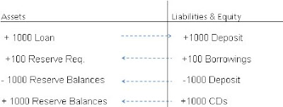
However, in the real world, money is endogenously created. Banks do not passively await funds to issue loans. Banks extend loans to creditworthy borrowers to meet the needs of trade. In this process, loans create deposits and deposits create reserves. We can illustrate this using T-account as follows:
The bank makes a new loan (+1000) and at the same time the borrower’s account is credited with a deposit of an equivalent amount of the loan. Thus, “the increase in the money supply is a consequence of increased loan expenditure, not the cause of it.” (Kaldor and Trevithick, 1981: 5)
In order to meet reserve requirements, banks can obtain reserves in secondary markets or they can borrow from Fed via the discount window.
As noted by Kaldor (1985), Minsky (1975), Goodhart (1984), Moore (1988), Wray (1990), Lavoie (1984) to name a few, money is endogenously created. The supply of money responds to changes in the demand for money. Loans create deposits and deposits create reserves as explained here and here. It turns the deposit multiplier on its head. Goodhart (1994) observed that “[a]lmost all those who have worked in a [central bank] believe that [deposit multiplier] view is totally mistaken; in particular, it ignores the implications of several of the crucial institutional features of a modern commercial banking system….’ (Goodhart, 1994:1424).
As Fulwiller put it, “deposit outflows, if they exceed the bank’s RBs, result in overdrafts. Banks clear this via lowest cost available in money markets or from the Fed.” In this case, let us assume that the bank issues some other liability, such as CDs, in order to obtain the 1000 reserves needed for clearing its overdraft at the Fed.
It reverses the orthodox story of the deposit multiplier (M=mB). Banks are accepting the liability of the borrower and they are creating their own liability, which is the demand deposit. In this process, banks create money by issuing its own liability, which is counted as a component of the money supply. Banks do not wait for the appropriate amount of liquid resources to exist to provide new loans to the public. Instead, as Lavoie (1984) noted ‘money is created as a by-product of the loans provided by the banking system’. Wray (1990) puts it best:
“From the bank’s point of view, money demand is indicated by the willingness of the firm to issue an IOU, and money supply is determined by the willingness of the bank to hold an IOU and issue its own liabilities to finance the purchase of the firm’s IOU…the money supply increases only because two parties willingly enter into commitments.” (Wray 1990 P.74)
As showed above, when banks, overall, are in need of more high-powered money (HPM), they can increase their borrowings with the central bank at the discount rate. Reserve requirements (RRs) cannot be used to control the money supply. In fact, RRs increase the cost of the loans granted by banks. As Wray pointed out “in order to hit the overnight rate target, the central bank must accommodate the demand for reserves—draining the excess or supplying reserves when the system is short. Thus, the supply of reserves is best characterized as horizontal, at the central bank’s target rate.” The central bank cannot control even HPM!The latter is provided through government spending (or Fed lending). The central bank can only modify its discount rate or its rate of intervention on the open market.
Bernanke is concerned that the sharp increase in reserve balances “would produce faster growth in broad money (for example, M1 or M2) and easier credit conditions, which could ultimately result in inflationary pressures.” He is considering the money-price relationship given by the old-fashioned basic quantity theory of money relating prices to the quantity of money based on the equation of exchange (The idea that money is related to price levels and inflation it is not a new idea at all, you can find that, for example, in Hume and other classical economists):
M*V = PQ, where M stands for the money supply (which in the neoclassical model is taken as given, i.e. exogenously determined by monetary policy changes in M), Q is the level of output predetermined at its full employment value by the production function and the operation of a competitive labor market; P is the overall price level and V is the average number of times each dollar is used in transactions during the period. Causality runs from the left-hand side to the right-hand side (nominal output)
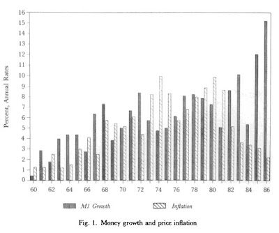
According to the monetarist view, under given assumptions, changes in M cause changes in P, i.e. the rate of growth of the money supply (such as M1 and M2) determines the rate of change of the price level. Hence, to avoid high inflations monetary policy should pursue a stable low growth rate in the money supply. The Fed, under Paul Volcker, adopted money targets in October 1979. This resulted in extremely high interest rates, the fed-funds rate was above 20%, the US had double digit unemployment and suffered a deep recession. In addition, the Fed did not hit its money targets. The recession was extremely severe and in 1982 Volker announced that they were abandoning the monetarist experiment. The rate of money growth exploded to as high as 16% p.y, over 5 times what Friedman had recommended, and inflation actually fell (see figure below).
Source: Benjamin Friedman, 1988 :55
The Collapse of the Money-Income and Money-Price Relationships
A closer look at the 1980s and 1990s help us understand the relationship between monetary aggregates such as M1 and M2 and inflation. This is a relationship that did not hold up either in the 1980s nor in the 1990s. As Benjamin Friedman (1988) observed “[a]nyone who had relied on prior credit-based relationships to predict the behavior of income or prices during this period would have made forecasts just as incorrect as those derived from money-based relationships.” (Benjamin Friedman, 1988:63)
Despite the collapse of the relationship between monetary aggregates and inflation Bernanke still believes that “we must either eliminate these large reserve balances or, if they remain, neutralize any potential undesired effects on the economy.” He noted that “we will need to tighten monetary policy to prevent the emergence of an inflation problem down the road” However, is inflation always and everywhere a monetary phenomenon? The answer is no. The picture below plots the credit-to-GNP ratio. Note that even “the movement of credit during the post-1982 period bore no more relation to income or prices than did that of any of the monetary aggregates.” (Benjamin Friedman, 1988:63, emphasis added)
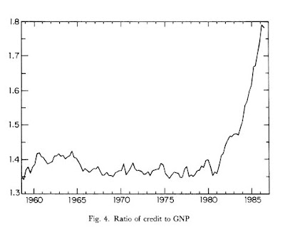
What about the other monetary aggregates? Benjamin Friedman (1988) pointed out that “[t]he breakdown of long-standing relationships to income and prices has not been confined to the M1 money measure. Neither M2 nor M3, nor the monetary base, nor the total debt of domestic nonfinancial borrowers has displayed a consistent relation- ship to nominal income growth or to inflation during this period.” (ibid, p.62)
Even Mankiw admitted that “[t]he standard deviation of M2 growth was not unusually low during the 1990s, and the standard deviation of M1 growth was the highest of the past four decades. In other words, while the nation was enjoying macroeconomic tranquility, the money supply was exhibiting high volatility. The data give no support for the monetarist view that stability in the monetary aggregates is a prerequisite for economic stability.” Mankiw, 2001: 33)
He concluded that “[i]n February 1993, Fed chairman Alan Greenspan announced that the Fed would pay less attention to the monetary aggregates than it had in the past. The aggregates, he said, ‘do not appear to be giving reliable indications of economic developments and price pressures’… [during the 1990s] increased stability in monetary aggregates played no role in the improved macroeconomic performance of this era.” (Mankiw 2001, 34)
A recent study conducted by the FRBSF also concluded that “there is no predictive power to monetary aggregates when forecasting inflation.” What about the Japanese experience? As the figure below shows, the monetary base exploded but prices actually fell!
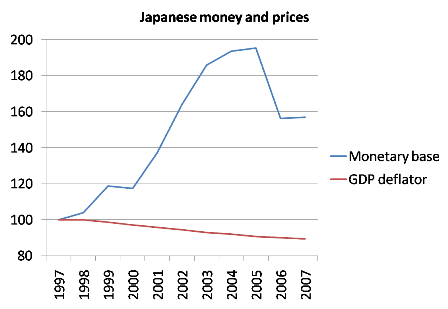
Source: Krugman
What about the US in the 1930s? The same pattern happened, HPM rose sharply and prices were stable!
Source: Krugman
Chairman Bernanke should learn the basic lesson that money is endogenously created. Money comes into the economy endogenously to meet the needs of trade. Most of the money is privately created in private debt contracts. As production and economic activity expand, money expands. The privately created money is used to transfer purchasing power from the future to the present; buy now, pay latter. It allows people to spend beyond what they could spend out of their income or assets they already have. Money is destroyed when debts are repaid.
Consumer price inflation pressures can be caused by struggles over the distribution of income, increasing costs such as labor costs and raw material costs, increasing profit mark-ups, market power, price indexation, imported inflation and so on. As explained above, monetary aggregates are not useful guides for monetary policy.
David Henderson & Jeff Hummel argued against George Selgin that a volatile velocity offsetting a volatile money supply is just what we'd expect (desire) if it is meeting demand and producing stability.Mike Sproul has recently been arguing against the quantity theory of money in favor of the "backing theory" of the Real Bills Doctrine in the comments at The Money Illusion. He also promotes it on his won faculty page, but the running conversation is at Scott's.Scott noted that Joan Robinson claimed Weimar Germany did not have a loose money policy, as a synechdoce for those silly Post Keynesians. I know there are some advocates of PK here and wondered what you think of that.
I agree the conventional “textbook” presentation of the “money multiplier” portrays an erroneous causality between reserves and deposits – i.e. the correct causality is that central banks supply reserves in response to the process whereby commercial banks create money by extending credit. Reserve requirements are not generally binding on the ability of the banking system to create money and credit. Central banks change interest rates when they think the credit/money process requires it, among other reasons. This is all to say that excess reserves are not a necessary condition for the expansion of credit and money.However, this does not mean that excess reserves have absolutely no effect on the expansion of credit and money.You would have a hard time convincing me that an excess reserve position of X + 1 has precisely the same effect on a commercial bank’s asset strategy as an excess reserve position of X. As a matter of fact, individual bank reserve managers do respond to the distribution of available system reserves in normal times. An individual bank with X or X + 1 in excess reserves will definitely consider that position in its own reserve management and money market operations. It may well purchase treasury bills as a result. Those bills may be sourced from the non-bank sector, in which case new money will be created.Of course, the central bank normally holds the system excess reserve setting at a fairly tight level in order to avoid transmitting this sort of signal to the banking system as a whole, willy-nilly. So the distribution effect I’ve described among individual banks tends to ebb and flow, back and forth, with no real permanent effect on asset expansion.But the point is that the conventional textbook causality is still possible, whereby the banking system responds to excess reserves supplied by the central bank, IN ADDITION to the normal process whereby the central bank responds to banking system balance sheet expansion by supplying the resulting required reserves. The textbook described causality remains wrong in the sense that it is reversed from what is applicable in a normal excess reserve environment. But this does not mean it cannot occur in an abnormal excess reserve environment.In this sense, you and Bernanke are both right.That said, Bernanke’s reference to the possibility of this scenario is too simplistic. The subject of the potential banking system response to excess reserves requires a coherent analysis of the interaction between bank liquidity (in the form of excess reserves) and bank capital (in the sense of support for bank balance sheet expansion generally). Indeed, the subject of monetary theory suffers from a lack of integration with the role of bank capital adequacy in the creation of credit and money.
Really liked the blog post. Figure 3 really says it all! Hits the nail on the head. In fact reminds of Galileo's Leaning Tower of Pisa Experiment. Unfortunately, Economists cannot do such experiments. However the blogosphere is a powerful medium to convey your knowledge. Even the Chicago Fed's Modern Money Mechanics says how banks expand their balance sheets. If Ben Bernanke happens to read this post and doesnt believe it, he should read the Chicago Fed publication.
Hi JKHThere's a big difference between saying that ER affect a bank's asset allocation and saying that it affects their lending standards. We argue the latter is incorrect, not the former. Certainly a bank with undesired ER tries to get rid of them . . . we've always said that. But this means substituting them for other short-term assets that earn a market return. Again, we've always acknowledged that, as does everyone else doing research in this area. That's precisely why CBs drain undesired excess balances . . . banks try to get rid of them otherwise and can't before the overnight rate falls below the CBs target. This doesn't mean, though, that the bank would be more willing to lend to a would-be purchaser of a home or car as he/she walks through the bank's front doors just because it has more ER . . . and as you already know, the ER don't give it any more ability to make that loan, either.Best,Scott
Thanks, Scott.Really good post by Felipe, BTW.
Thanks for admonishing Bernanke. He has a Ph.D from MIT, was Phi Beta Kappa, & is FED Chairman. 1) "banks should find more opportunities to lend out their reserves"(2) "because banks will not want to lend out their reserves"Member banks do not loan out excess reserves. CBs are unemcumbered in their lending operations. Excess Reserves are earning assets. But lower the remuneration rate and the competitive advantage vis a' vis the effective FFR disappears.The "monetary base" is not a base for the expansion of money & credit. Between 90-47 percent has been currency held by the non-bank public. Currency has no expansion coefficient. 1/2 the base [sic] is currency & 1/2 of M1 is currency. (cum hoc ergo propter hoc)& "the demand for money" There is no such thing as a liquidity preference curve. Money thus is a paradox – by wanting more, the public ends up with less, and by wanting less, it ends up with more (Alfred Marshall). Therefore the money supply can never be managed by any attempt to control the cost of credit.
The transactions concept of money velocity (Vt) has its roots in Irving Fischer’s equation of exchange (PT = MV), where (1) M equals the volume of means-of-payment money; (2) V, the rate of turnover of this money; (3) T, the volume of transactions, and P, the average price of all transactions units. The real impact of monetary demand on the prices of goods and serves requires the analysis of “monetary flows”, and the only valid velocity figure in calculating monetary flows is Vt. Income velocity (Vi) is a contrived figure (Vi = Nominal GDP/M) (as opposed to Milton Friedman WSJ, Sept. 1, 1983). The product of MVi is obviously nominal GDP. So where does that leave us?… In an economic sea without a rudder or an anchor. A rise in nominal GDP can be the result of (1) an increased rate of monetary flows (MVt) (which by definition the Keynesians have excluded from their analysis), (2) an increase in real GDP, (3) an increasing number of housewives selling their labor in the marketplace, etc. The income velocity approach obviously provides no tool by which we can dissect and explain the inflation process.To the Keynesians, aggregate demand is nominal GDP, the demand for serves (human) and final goods. This concept excludes the common sense conclusion that the inflation process begins at the beginning (with raw material prices and processing costs at all stages of production) and continues through to the end. But we do know that to ignore the aggregate effect of money flows on prices is to ignore the inflation process. And to dismiss the concept of Vt by saying it is meaningless (that people can only spend their income once) is to ignore the fact that Vt is a function of three factors: (1) the number of transactions; (2) the prices of goods and services; (3) the volume of M. Inflation analysis cannot be limited to the volume of wages and salaries spent. To do so is to overlook the principal "engine" of inflation – which is of course, the volume of credit (new money) created by the Reserve and the commercial banks, plus the expenditure rate (velocity) of these funds.Also overlooked is the effect of the expenditure of the savings of the non-bank public on prices. The (MVt) figure encompasses the total effect of all these money flows.Some people prefer the devil theory of inflation: “It’s peak oil’s fault or peak debts fault.” This approach ignores the fact that the evidence of inflation is represented by “actual” prices in the marketplace. The “administered” prices of the world’s oil producing countries, would not be the “actual” market prices, were they not “validated” by (MVt), i.e., “validated” by the world’s central banks."Volker announced that they were abandoning the monetarist experiment" Volcker targeted non-borrowed reserves when at times 10% of all reserves were borrowed. One dollar of borrowed reserves provides the same legal-economic base for the expansion of money as one dollar of non-borrowed reserves. Coincident with the DIDMCA legal reserves exploded from April 1st until Dec 31 at a 13.3% annual rate, etc., etc.
"Volker announced that they were abandoning the monetarist experiment" Volcker targeted non-borrowed reserves when at times 10% of all reserves were borrowed. One dollar of borrowed reserves provides the same legal-economic base for the expansion of money as one dollar of non-borrowed reserves. Coincident with the DIDMCA legal reserves exploded from April 1st until Dec 31 at a 13.3% annual rate, etc., etc.
First, there is no ambiguity in forecasts: In contradistinction to Bernanke (and using his terminology), forecasts are mathematically "precise” :(1) “Money” is the measure of liquidity; & (2) Income velocity is fabricated; it’s the transactions velocity (bank debits) that matters (financial transactions are not random);(3) Nominal GDP is measured by monetary flows: (MVt), i.e., our means-of-payment money (M), times its rate of turnover (Vt);(4) The rates-of-change (roc’s) used by economists are specious (always at an annualized rate; which never coincides with an economic lag). Friedman became famous using only half the equation (the means-of-payment money supply), leaving his believers with the labor of Sisyphus.Contrary to economic theory, and Milton Friedman, monetary lags are not “long and variable”. The lags for monetary flows (MVt), i.e. proxies for (1) real-growth, and (2) inflation, are historically, always, fixed in length. However the lag for nominal gdp varies widely.Roc’s in (MVt) are always measured with the same length of time as the specific economic lag (as its influence approaches its maximum impact; as demonstrated by the clustering on a scatter plot diagram).Not surprisingly, adjusted member commercial bank “free" legal reserves (their roc’s), corroborate both lags for monetary flows (MVt) their lengths are identical (as the weighted arithmetic average of reserve ratios remains constant).The lags for (1) monetary flows (MVt), & (2) "free" legal reserves, are synchronous & indistinguishable. Consequently, this makes economic forecasting automatically, mathematically, infallible (for less than one year). Economic bubbles are obvious. The BEA uses quarterly accounting periods for real GDP and the deflator. The accounting periods for GDP should correspond to the specific economic lag, not quarterly. Monetary policy objectives should not be in terms of any particular rate or range of growth of any monetary aggregate. Rather, policy should be formulated in terms of desired roc’s in monetary flows (MVt) relative to roc’s in real GDP. Note: roc’s in nominal GDP can serve as a proxy figure for roc’s in all transactions. Roc’s in real GDP have to be used, of course, as a policy standard. Because of monopoly elements, and other structural defects, which raise costs, and prices, unnecessarily, and inhibit downward price flexibility in our markets, it is probably advisable to follow a monetary policy which will permit the roc in monetary flows to exceed the roc in real GDP by c. 2 – 3 percentage points. I.e., monetary policy is not a cure-all, there are structural elements in our economy that preclude a zero rate of inflation. In other words, some inflation is inevitable given our present market structure and the commitment of the federal government to hold unemployment rates at tolerable levels.