Tag Archives: The Federal Government Deficit

Another Take on the Financial Balances

By Eric Tymoigne

First, regarding the identity itself, for a domestic economy we have, in terms of economic flows:

GFB + PDFB + RWFB ≡ 0

With PDFB the private domestic financial balance, RWFB the financial balance of the Rest of the World, and GFB the government financial balance. This identity holds all the time, in any domestic economy (in a world economy RWFB disappears). For economic analysis, it is insightful to arrange this identity differently in function of the type of monetary regime.
In a country that is monetarily sovereign the federal government has full financial flexibility. By monetary sovereignty, one means that there is a stable and operative federal/national government that is the monopoly supplier of the currency used as ultimate means of payment in the domestic economy, and that the domestic currency is not tied to any asset (like gold) or foreign currency. Other posts have already explained the implications of this in terms of federal government finance (taxes and T-bonds do not act as financing sources for federal government spending, the federal government always spends by creating monetary instruments first, etc.) and banking (bank advances create deposits, credit supply is endogenous and is created ex-nihilo (i.e. banks do not need depositors to be able to provide an advance of funds to deficit spending units), higher reserve ratios do not constrain directly the money supply process in a multiplicative way, etc.). All this also has implications in terms of accounting and in terms of modeling.

First, in terms of accounting identity, in a monetarily sovereign country, the government financial balance (GFB), through the federal government financial balance, is the ultimate means to accommodate the changes in holdings of the domestic currency by other sectors (private domestic sector and the Rest of the World). This means that, for a monetarily sovereign country, the most insightful way to arrange the national accounting identity is:

-GFB ≡ PDFB + RWFB

or

-GFB ≡ NGFB

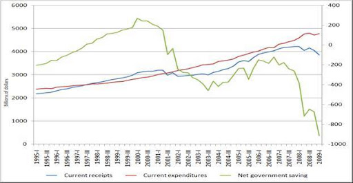
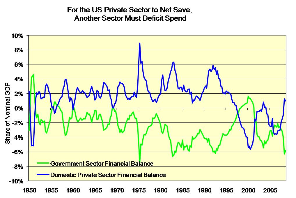
Where NGFB is the non-government financial balance (the sum of the financial balance of the private domestic sector and the Rest of the World). This way of arranging the identity shows well that the government sector (through its federal branch) is the ultimate provider/holder of domestic currency: government fiscal deficit (surplus) is always equal to non-government financial surplus (deficit). The graph below shows the identity for the US.

Fiscal balances for the United State (billions of dollars)

Source: BEA (Table 5.1).
Note: Statistical discrepancy was distributed evenly among the three sectors (Private Domestic, Rest of the World, and Government).

Any net injection of dollars (i.e. financial deficit) by any sector must be accumulated somewhere else (i.e. financial surplus). As the monopoly supplier of ultimate domestic means of payment, usually the US government sector is the net injector of dollars, while the private domestic sector and the Rest of the World usually accumulate the dollars injected. For a while, like from 1997 to 2007 in the US, the private domestic sector and the Rest of the World may transfer the domestic currency among each other while the government runs a surplus; however, this cannot last because ultimately one of them (private sector or Rest of the World) will run out of domestic currency and/or will have to become highly indebted in domestic currency leading ultimately to a Ponzi process that collapses. Only the federal government has a perfect creditworthiness and can always meet its financial obligations denominated in the domestic currency (that is why US Treasury bonds are not rated, default rate is zero).

In addition, one may note that the Rest of the World and the private sector cannot accumulate any domestic currency unless the government sector injects them in sufficient quantity in the first place. Stated alternatively, the Rest of the World (e.g., the Chinese) does not help to finance the deficit of the federal government (US federal government). On the contrary, the federal government deficit allows the Rest of the World to accumulate dollars. This pressure to generate a deficit is all the more strong on the dollar that it is the reserve currency of the world, so there is a net demand for the dollar from the Rest of the World.

This also works the other way around, i.e. if the Rest of the World disaccumulates the domestic currency the government must be the ultimate acquirer of this domestic currency and so must run a surplus if the private domestic sector does not accumulate it in a large enough quantity.
Once it acquires the domestic currency, the government may destroy them (federal government has huge shredders or they are deleted from the computer memory), or store them into a safe/computer for later use (especially true for state and local governments). Destruction of bank notes occurs usually because they are in bad shape. Hundreds of millions of dollars worth of bank notes are destroyed every month at the Fed banks in the US; then they are used as compost (during my last tour of the San Francisco Fed last March, I was told that about $56 million worth of bank notes are destroyed every day at the SF Fed, and then are spread on the fields of California). If you go visit a fed bank this will be the main attraction.

Besides the poor condition of some bank notes, the destruction of dollars by the federal government may also occur for other reason, e.g., because there is a lack of storage capacity (safe is too small, computer memory is too small). One central point is that the dollars that are accumulated by the federal government do not increase its financing capacity because the federal government created those dollars in the first place. It chooses not to destroy them all because it takes time and it is costly to destroy and to make monetary instruments, and because it has the storage capacity.

For the moment, we stayed at the level of the identity, which basically tracks where the domestic currency comes from and where it goes. Every dollar comes from somewhere and must go somewhere. There is no dollar floating around that is not held by a sector. No desire/behavioral equation were included in the analysis above. However, even that basic identity provides us a powerful insight. Indeed, it shows us that it is impossible for all sectors to be in surplus; at least one of them must deficit spend and usually it is the government sector because of its monetary sovereignty. The reverse is also true, i.e. not all sectors can be in deficit at the same time; at least one of them must be in surplus (usually the private domestic sector). As Randy noted in a previous post, this is probably not understood well; even the Wall Street Journal did not make the connection in early the 2000s between the federal government surplus and the households’ negative saving. It is often assumed that if they wish, all sectors could be in surplus; one just needs to work hard enough at it (note that this is one of the promises that is always made during presidential campaigns: “we should save more, reduce our trade deficit and reach a fiscal surplus”). Economic reality does not work that way.

In terms of the model (where one includes desires and so behavioral aspects as well as an explanation of the adjustment mechanisms to those desires in relation to the state of the economy), for the analysis of a monetarily sovereign country, I would rather put the desired financial balance of the Rest of the World with the desired private domestic financial balance and call the sum the desired financial balance of the non-government sector (NGFBd). The model does not deal with stocks at all and their relation to flows (IS-LM did try but failed to do it correctly; read Hicks’s own account in his JPKE article “IS-LM: An explanation”); however, the financial-balance model is a good place to start in Econ 101. If students can understand the model, the identity and how they relate to each other, it would be a HUGE step forward in terms of removing this counterproductive phobia of government fiscal deficits (then one would have to learn about government finance and the monetary creation process, which, like many other things, are all taught backward in textbooks).

If the Rest of the World has too many dollars relative to its taste it and cannot bring them back into the domestic economy, by buying enough goods and services or financial assets from the private domestic and government sectors, the currency depreciates and/or long-term interest rate falls. This boosts exports and reduces imports. This may also promote investment and consumption if the state of expectations is stable.

If the non-government sector desires to save more, then, unless the government sector increases its spending propensity or reduces tax rates, the economy will enter a slump; possibly a debt-deflation process if debt levels are far too high. All this was done nicely in previous posts.
Before, during, and after the adjustment processes (variation of flows, levels and prices) the identity holds and the actual financial balance always sum to zero. The sum of GFBd and NFGBd will be different from zero except when the adjustment is completed, i.e. when actual and desired balances are equal (“at equilibrium” if you want to call it that way, even though markets may not be cleared).

The Sector Financial Balances Model of Aggregate Demand

By Scott Fullwiler

Paul Krugman’s recent post indicates that perhaps those of us taking a stock-flow consistent approach to macroeconomics may be making some headway. My fellow blogger, Rob Parenteau, and another friend, Bill Mitchellboth describe many of the details of this approach and how they fit the graph posted by Krugman. Rob is correct to suggest this would be a much better framework for understanding macroeconomics than the traditional IS-LM model, which was highly flawed to begin. My purpose here is to build on both of these posts and demonstrate a few uses of the model (thus, those not familiar with this framework should read Rob’s and/or Bill’s posts first, probably).To begin, consider the graph in Krugman’s post below:

Continue reading

Employing Krugman’s Cross: Farewell, Mr. Hicks?

By Robert Parenteau

Paul Krugman’s July 15th blog post diagramming financial balances makes some important steps in revealing the analytical power of the financial balance approach to macroeconomics – something once understood by J.M Keynes and early Keynesians like Nicholas Kaldor, Abba Lerner, and Joan Robinson, but long since lost in the headlong rush over the past three decades of mainstream macroeconomics to become a special branch of microeconomics, which itself appears to have become a special branch of applied calculus in some sort of rather twisted physics envy. I suspect reading Minsky has helped Paul immeasurably in seeing these relationships, and I would urge him and others to go find some of Wynne Godley’s contributions (many of which are available online at the Levy Economics Institute) to a stock/flow coherent macroeconomics, and it may all become that much clearer.

The diagram Paul presented at first (reproduced below) threw me for a loop, but I believe I now see what he was doing, as the labeling did not initially make it clear, and perhaps by walking through Paul’s diagram, others can avoid my initial confusion.


The upward sloping line should be labeled the private sector financial balance (PSFB), and the downward sloping line should be labeled the government financial balance (GFB). Only the part of the PSFB schedule above the horizontal axis is in surplus, if this horizontal GDP axis crosses the vertical sectoral financial balance axis at zero. Similarly, only that part of the GFB schedule above the horizontal axis is in deficit. I believe Paul has defined the vertical axis such that the range above zero represents a rising PSFB, and at the same time, a falling GFB of the same absolute amount, but of opposite sign. Then the area below zero is a falling PSFB and a rising GFB. Above zero represents a private sector financial surplus and a government deficit, while below zero represents a private sector deficit and a government surplus.

Confusing at first, but this follows because Paul has simplified the analysis to two sectors, and sectoral financial balances must balance ex post for any accounting period. The range above zero representing a private sector surplus must also represent a government deficit (GFB must be of equal magnitude but opposite sign to the PSFB). This would seem consistent with Paul’s GFB schedule falling below zero as GDP increases, since a falling fiscal deficit would eventually give way to an increasing fiscal surplus as income increases if automatic stabilizers work as we believe they do (see previous post here). Similarly, the rising PSFB schedule is consistent with traditional Keynesian stability conditions, with saving increasing faster in income than investment does, although we should all keep in mind, as Minsky emphasized, that explosive growth dynamics (Minsky’s upward instability) can arise in economic expansions characterized by euphoric asset pricing. Hence, the last two US business cycle expansions have been characterized by a falling PSFB (that is, deficit spending by the household and business sectors combined), not a PSFB rising as income rises, but that can be accommodated in less simplified versions of Krugman’s cross.

Another way to see why this interpretation of the diagram must be correct is that when the PSFB schedule shifts up and to the left, representing a higher desired net private saving at each level of income, the new point of intersection with the GFB schedule would, for example represent a new short run equilibrium point where say a $250b net private saving position is met by a $250b fiscal deficit. Again, sectoral financial balance must balance ex post (as explained in prevoius posts here and here). If one sector is running a net saving or surplus position, the other sector must be dissaving or deficit spending. That is the tyranny of double entry book keeping – not high Keynesian theory.

If I now have the orientation of the diagram straight in my head (and this is the only way I can see that it makes sense), those who believe in fiscal rectitude may wish to notice two aspects of the world we live in. If you view a balanced fiscal budget as the ultimate and over riding goal, you can get there one of two ways from Paul’s second PSFB schedule (the higher line we seem to have shifted to, as asset prices and profitability have collapsed over the past year, thereby forcing lower private investment and driving saving out of private income flows higher).

To arrive at a fiscal balance, you can shift the GFB schedule down and to the left by jamming tax rates higher and lowering the government spending propensities out of tax revenue income until the GFB schedule intersects the PSFB schedule at the point where the PSFB schedule crosses the horizontal axis at the zero financial balance mark. Notice the level of income the economy is then operating at, and all of you who pay dues to the Concord Coalition, please consider whether existing private debt loads could actually be serviced at that lower level, since most private debt contracts are fixed nominal payment commitments. Think post Lehman bankruptcy, on steroids, and you might get a taste of what you are praying for with perpetually balanced fiscal budgets.

The second way to get to a fiscal balance is to encourage the PSFB schedule to shift down and to the right until it intersects the GFB schedule at the point at which it crosses the horizontal axis. That means increasing incentives for the private sector to invest more money at each income level and save less money at each income level. Given the residential housing stock overhang, and the need for households to save out of income flows if they cannot rely on serial asset bubbles to deliver the appropriate nominal net worth at retirement, that means ways must be found to encourage US businesses to pursue a higher reinvestment rate in the US, rather than borrowing money to buy back shares to boost stock prices or reinvesting abroad. Not easy, but not impossible either. Notice also that the second form of adjustment leaves you at a higher equilibrium income level, and the existing private debt to GDP ratio will stabilize, since there will be no additions to the private debt stock, as net private deficit spending is zero at the new income flow level.

Of course, this should all eventually be recast in dynamic terms. For example, income won’t grow unless the GFB is continually shifting up and to the right, or the PSFB is continually shifting down and to the right (or some combination of the two). There is also no obvious endogenous mechanism shifting the PSFB toward a position of full employment income over time, given the position of the GFB. Of course, in theory, policy could be geared such that given reasonable estimates of the likely position of the PSFB schedule, the GFB schedule could be shifted out (or less likely, in) to achieve the level of income associated with full employment. Alternatively, fiscal policy could be structured so the GFB schedule could be perfectly vertical at the full employment level of income, which in many ways is what an employer of last resort (ELR) driven fiscal policy attempts to do.

Finally, for those insistent that public and private debt to income ratios must be held fixed from here to eternity for whatever reason, then starting from Paul’s initial equilibrium, income growth could only be accomplished if the PSFB schedule could be encouraged to shift outward, and the GFB could be shifted in concert such that either the realized financial balances of both sectors were kept at zero, or there was some cycling between the two, such that periods of private sector financial deficits were followed by periods of government sector deficits of similar magnitude and duration.

The trade balance must also be brought back into the story, as a trade surplus is the only way both the GFB and the PSFB can maintain a net saving position at the same time (assuming for whatever reason that was a worthy goal), but at least it is a promising start at representing how sectoral financial balances are related, and it reveals many of the misconceptions that unnecessarily cloud the debate.

If the Krugman Cross does nothing more than provide a stepping stone away from the dead end trap of the Hicks/Harrod/Meade IS/LM diagram, then this is a useful initial contribution. Caught under the spell of IS/LM conventions, Paul and other New Keynesians have spilled far too much ink trying to devise ways of instituting negative real interest rates to get the economies out of a balance sheet driven recession. With policy rates near zero, this analysis has devolved into arguments about how best to increase inflation expectations or actual inflation in order to achieve a sufficiently negative real interest rate. From a practical point of view, the last thing households facing heavy debt servicing loads with falling wage and salary incomes need are rising consumer prices that drain their already reduced discretionary income. Households need higher money incomes, not higher consumer prices, expected or actual, to exit their current difficulties. Real interest rates are diversion from the real problem at hand in a balance sheet recession, which is how to get the economy to a point where money income levels can service most private debts. Krugman’s Cross makes it obvious – shift the GFB schedule in response to shifts in the PSFB schedule.

As always, we must be careful about sliding between the usual ex ante/ex post distinctions, as the income multiplier lies masked behind these interactions, as does the reconciliation of new liability issuance with portfolio preferences, among other balance sheet and asset price considerations that must be brought into play for a coherent stock/flow macroeconomics, of which Hick’s IS/LM approach was a pale shadow that concealed more than it revealed.

For example, the private sector may plan to net save more at any given expected income or GDP level, but unless some other sector net saves less or deficits spends more, private incomes will adjust downward, and the desired private net saving will be thwarted, paradox of thrift style. If Paul recalls his reading of Keynes’ General Theory (and he is to be applauded for being one of the few New Keynesians to actually read Keynes in the original), this is one of the reasons Keynes argues incomes adjust to close gaps between intended investment and planned saving. Interest rates do not equilibrate investment and saving – incomes do, in Keynes’ General Theory. Paul has taken a very large step in this direction with his financial balance diagram, which hopefully he will find more powerful than his IS/LM analytics which he employed in the case of the Japanese balance sheet recession.

Specifically, Paul refers to the need for net private saving being “absorbed” by the public deficit spending. That assumes the net private saving can exist without some other sector deficit spending at the same time, which is impossible. William Vickrey and James Tobin used to make a similar slip, with Vickrey arguing the private saving had to be recycled by public deficit spending (see Vickrey’s otherwise useful piece on 15 fundamental fallacies, linked at CFEPS here.

In Paul’s 2 sector model, unless the public sector spends more money than it takes in as tax receipts, the private sector cannot earn more money than it spends, no matter what its plans or intentions or ex ante designs. Net private saving is created, allowed, or constrained by the size of the public deficit. Net private saving cannot exist as anything more than a hope and a prayer unless some other sector is willing and able to deficit spend. Ex post, in a 2 sector model, as a matter of basic accounting, the net saving of one sector must be equal to the net deficit spending of the other. That is the short run accounting “equilibrium” or reality.

Moving beyond a simple 2 sector model to the world we actually inhabit, it is really as simple as this. The US household sector cannot net save in nominal terms (spend less money than it earns) unless some other sector (or combination of sectors) is willing and able to spend more money than it earns.

It can be the government, the business, or the foreign sector or some mix of the three that net deficit spends – take your choice. But keep in mind, of the three, a government with a sovereign currency (not convertible into fixed quantities of a commodity or another currency on demand) and no debt denominated in foreign currencies is the only one of those three that cannot go bankrupt and cannot default on its debt while continuously deficit spending – unless it chooses to default for some odd political reason.

The sooner we face this fundamental reality of contemporary monetary and economic arrangements, the better. It does not require swearing allegiance to high Keynesian theory – it is simply an accounting reality. Reject it, and you will also have to throw at least seven centuries of double entry book keeping out the window as well.

Since the US economy does appear to have entered a debt deflation spiral for the first time in a lifetime, and it does appears that the spiral has been contained for the moment by a reduction in the trade deficit and a surge in the fiscal deficit, it might be a good time for economists, investors, policy makers, and the general public to once and for all find some clarity on these questions regarding financial balances and the economy. Perhaps Paul’s simple back of the napkin diagram of financial balances takes us one step in that direction.

A note on Automatic Stabilizers

What has so far prevented a deep depression in 2009? The answer, as Paul Krugman explained yesterday, are automatic stabilizers. Indeed, as Hyman Minsky emphasized more than 20 years ago in his book Stabilizing an Unstable Economy (1986), this feature of the federal government’s budget – i.e. the fact that it moves counter-cyclically in an automatic fashion – imparts a great stabilizing force to aggregate demand.

The figure below sheds light on the non-discretionary (i.e. automatic) nature of government deficits. In an economic downturn, tax receipts automatically fall, and government expenditures automatically rise, resulting, automatically, in budget deficits. (net govt saving = right hand scale)

Source: Bureau of Economic Analysis (BEA)

The components of government spending that rise automatically are called ‘transfer payments’, that include unemployment compensation, Medicaid, grants-in-aid to state and local government, etc.
With these forms of payment increasing and tax receipts declining due to falling economic activity, the federal budget moves automatically into deficit.

Source: Bureau of Economic Analysis (BEA)

So far the stimulus package was not what saved the US economy. The budget projections show that 24% of the total cost of the stimulus package will occur in fiscal year 2009 (which means $198 billion) and 47% of it occurring in fiscal year 2010.

“The ARRA is estimated in the budget to cost $825.4 billion over the next 10 years. These costs are split between $600.0 billion in increased outlays and $225.4 billion in reduced receipts. Although the cost of the ARRA is spread over 10 years, the budget projections show 24 percent of the total cost occurring in fiscal year 2009 and 47 percent of the total cost occurring in fiscal year 2010…The budget estimates that receipts will be reduced $77.4 billion in fiscal year 2009 and $152.3 billion in fiscal year 2010 primarily because of the tax provisions of ARRA… The budget estimates that outlays will be increased about $120.2 billion for fiscal year 2009 and $237.8 billion for fiscal year 2010 because of the spending and investment provisions of the ARRA.”

As noted in previous posts (here, here, and here), government deficits, themselves, perform an important stabilizing function, because they allow the private sector to net save. Given that during a recession there is a sharp increase in uncertainty and insecurity, the private sector desires to spend less than its income which translates into a rising personal saving rate. In the current recession, the forecast is that the personal saving rate will reach 10% in 2009 and that jump to 14-16% by 2010. Such large decline in consumption means falling sales, production and further declines in GDP. As noted above, to meet the private sector rising saving desire the government should run bigger deficits to prevent a deflationary spiral.

Source: Jan Hatzius, Goldman Sachs

As Minsky emphasized, the problem, during the Great Depression, was that the government sector was too small relative to the rest of the economy; it couldn’t fill the demand gap and allow the private sector to save as much as it desired. In the absence of large enough automatic stabilizers to offset swings in private spending, GDP contracted to the point where desired net nominal saving equaled actual net nominal saving. Note that in second half of the last century, given the private sector’s desire to have positive net nominal saving, the US government normally ran budget deficits.

As Wray pointed out, “Since WWII we have had the longest depression-free period in the nation’s history. However, we have had nine recessions, each of which was preceded by a reduction of deficits relative to GDP.” This directly results from the impact of large swings in the federal government’s budget.

Automatic stabilizers work by putting a floor under aggregate demand, preventing a deflationary spiral, but they also put ceilings in place, as rapid economic growth translates into rising tax revenues which destroy income and temper the expansion. The impact of large automatic stabilizers explains why we can have a deep recession but not a Great Depression. As Wray noted:

“With one brief exception, the federal government has been in debt every year since 1776. In January 1835, for the first and only time in U.S. history, the public debt was retired, and a budget surplus was maintained for the next two years in order to accumulate what Treasury Secretary Levi Woodbury called “a fund to meet future deficits.” In 1837 the economy collapsed into a deep depression that drove the budget into deficit, and the federal government has been in debt ever since. Since 1776 there have been six periods of substantial budget surpluses and significant reduction of the debt. From 1817 to 1821 the national debt fell by 29 percent; from 1823 to 1836 it was eliminated (Jackson’s efforts); from 1852 to 1857 it fell by 59 percent, from 1867 to 1873 by 27 percent, from 1880 to 1893 by more than 50 percent, and from 1920 to 1930 by about a third. (Thayer 1996) The United States has also experienced six periods of depression. The depressions began in 1819, 1837, 1857, 1873, 1893, and 1929. Every significant reduction of the outstanding debt has been followed by a depression, and every depression has been preceded by significant debt reduction. Further, every budget surplus has been followed, usually sooner rather than later, by renewed deficits. However, correlation—even where perfect—never proves causation. Is there any reason to suspect that government surpluses are harmful?”

Gift-Wrapping the White House for the GOP

by Stephanie Kelton

It looks like Christmas has come early for one of President Obama’s most vocal critics. Rush Limbaugh said he hoped the president would fail, and the GOP is doing everything it can to make sure he does. The party stands united in its opposition to a (much-needed) ramping up of the federal stimulus effort. And, at the moment, the president is playing right into their hands.

Sen. Jon Kyl, R-Ariz., has called the $787 billion stimulus effort a “flop,” adding:

“The reality is, it hasn’t helped yet. . . Only about 6.8 percent of the money has actually been spent. What I propose is, after you complete the contracts that are already committed, the things that are in the pipeline, stop it.”

In other words, he thinks the stimulus isn’t working because the government isn’t spending the money FAST enough. And, with the lion’s share of the spending about to kick in, he wants to scrap the entire effort, just to make sure it won’t work.

The only thing more disappointing than hoping the president – any president – will fail is actively working to keep millions of Americans unemployed in order to score political points in the coming election. But that’s exactly what’s happening, and the president may be painting himself into a losing corner.

President Obama has insisted that: (1) the stimulus is working as planned; (2) a second stimulus is not needed; and (3) he will cut the deficit in half by the end of his first term.

If he sticks to his guns, I believe he will dig his own political grave (not to mention prolonging the agony for millions of Americans). He cannot have it both ways. He cannot reverse the effects of the worst economic downturn since the Great Depression and do it on a shoestring.

That isn’t to imply that $787 billion is chump change, but it pales in comparison to the losses that have already been borne by homeowners, businesses and investors. As Dean Baker recently pointed out, annual consumption is down about $700 billion (due to the loss of roughly $16 trillion in real estate and stock market wealth). Add to that “a reduction in annual rates of construction of about $450 billion” and a decline of “approximately $200 billion” in demand due to losses in the non-residential sector, and Baker says we’re looking at an annual loss of about $1,350 billion. And we’re trying to offset it with $300 billion or so (the annual stimulus) in spending by the federal government! It’s like using an umbrella to stop an avalanche. It won’t work.

But it gets worse, because Baker’s figures don’t account for the void that has been created by state and local governments, where expenditures have fallen by more than $64 billion in the last two quarters alone. And, with virtually every state bracing for even bigger cuts next year, we could easily lose another $100 billion or so in fiscal 2010. Then, of course, there’s the multiplier, which has been hard at work, exacerbating the magnitude of these cuts and costing us untold trillions in lost GDP.

But the president seems convinced that $787 billion will do the trick – at least according to his definition of the trick. You see, the Obama administration has not set the bar very high, and this seems to be why the president believes the stimulus has “worked as intended.” As he explained, it “wasn’t designed to restore the economy to full health on its own, but to provide the boost necessary to stop the free fall.” And this is why even bad news – e.g. 565,000 people filing first time jobless claims – can be interpreted as an indication that the stimulus is working as intended. (Recall that this was the smallest number since January 2009.)

Indeed, the president’s top economic advisors have always been careful to use the words “create or save” when describing the objective of the stimulus plan. And this means that net job creation isn’t the goal. The economy can continue to lose jobs faster than it creates them, and the policy will be described as “working” because the stimulus money helped at least some workers keep their jobs.

So the stimulus may be working “as intended,” but I don’t think the president can rely on semantics to carry him to victory in 2012. If President Obama wants a second term, he must join the growing chorus of voices calling for another stimulus and press forward with an ambitious program to create jobs and halt the foreclosure crisis. I have outlined my twelve-step recovery program, and others on this blog have put forward similar ideas. A payroll tax holiday that cuts FICA contributions to zero will provide immediate relief to millions of working families and their employers, boosting take-home pay as well as business profits. An additional $1,000 per capita will help ease the on-going budget crisis so that states can avoid further cuts to education and social services. A job-guarantee program, modeled on the WPA, will provide useful work and retraining opportunities for the many Americans who will not find jobs even after the economy recovers. Investing in our nation’s infrastructure – roads, bridges, transmission lines, etc. – will address years of neglect and improve the safety and security of all Americans.

These are the kinds of tangibles the American people will think about when they decide for themselves whether the stimulus was a success. At the end of the day, President Obama must cut loose the deficit bogy and abandon any date-specific goal for cutting the deficit in half. It is his Achilles heel. Let the deficit (and the debt) go where it will. With a sufficiently flexible fiscal response, GDP will explode, tax receipts will pour in, and the dreaded debt-to-GDP ratio will drop like a rock.

BerkShares, Buckaroos, and Bear Dollars: What Makes a Local Currency Tick?

by L. Randall Wray

Some commentators have argued that the proposed California “warrants” are similar to local currencies (see, e.g., Mark Thoma). In this piece I discuss experiments with local currencies and continue my argument that if California were to accept its own “warrants” in payment to itself, it could turn these into a functioning currency free of the defects of local currencies.

Interest in local currencies has soared in recent years, with nearly 100 U.S. communities experimenting with them. While proponents offer a variety of arguments in favor of local currencies, they share three common themes. First, there is concern that the use of a national, monopoly, currency creates a variety of economic, social, and environmental problems. Second, local currencies are said to improve regional communities, again across several dimensions including economic, social, political and environmental spheres. Third, many proponents want to reduce the power of national government, recognizing a relation between the monopoly of currency issue and centralization. They believe that decentralized money would shift power back to the communities.

At the same time, critics object that most local currency experiments quickly fail. Even the successful ones never displace local use of the national currency to any significant degree. Local currencies are inconvenient and appear to go against the prevailing tide of use of credit and debit cards rather than cash. Retailers must keep two sets of books, and many limit acceptance of local currencies to some kinds or amounts of purchases. Sales taxes must be paid in the national currency, so retailers must either collect taxes in the national currency, or pay taxes for the customers. In some cases, local currencies are accepted at a discount—with either the retailer or the customer bearing the cost. When the discount is borne by the retailer, businesses with low margins are reluctant to accept local currencies. Finally, in a national, and global, economy, most production and sales involve economic activities that are geographically dispersed–making it unlikely that local currencies can ever play much of a role.

The BerkShares program grew out of previous local currency systems used in the region. Local banks maintain a primary (currency exchange) market for BerkShares, selling and buying them for $0.90. Local merchants agree to accept BerkShares one-to-one against the dollar, effectively providing a ten percent discounted price. (This is because a customer can obtain one BerkShare for only ninety cents, purchasing an item priced at a dollar.) Merchants redeem excess BerkShares at participating banks at the fixed rate of one BerkShare equals ninety cents. Banks hold 100% dollar reserves against BerkShares issued, and absorb the cost of operating the exchange. Local consumers (and tourists) have a strong incentive to use BerkShares to take advantage of the ten percent discount; merchants have an incentive to accept them only if their sales increase sufficiently to offset the lost revenue due to the discount. This discount is treated as a business expense, much like a coupon or discounted sales price. There are now over 300 merchants participating and over 1.5 million BerkShares have been put into circulation.

A decade ago, the University of Missouri-Kansas City (UMKC) created a local currency, the Buckaroo (derived from slang for the dollar, “buck”, and from the University’s kangaroo mascot), with two purposes in mind: to teach students how a national currency “works”, and to provide community service to the Kansas City area. Most college students today are used to community service requirements, so the second objective could have been met by requiring that each student complete five service hours for every course. With 10,000 students enrolled in three courses each, 150,000 community service hours would be performed each semester—thereby accomplishing many of the community objectives identified above. However, we decided to provide more flexibility while enhancing the educational experience, so we created the Buckaroo. We provide to each community service organization as many Buckaroos it desires, stipulating that the provider pay only 1 Buckaroo per hour of labor.

Of course, on the first day of class when we tell students that they can earn Buckaroos by working at local charities, they invariably ask “but why do I want Buckaroos?”. The answer is that each student faces a 5 Buckaroo tax, which must be paid before the student can pass. Students are free to beg, borrow, earn, or exchange dollars (or any other valuables) to obtain the required Buckaroos. The vast majority of them choose to work with local community service providers to earn their Buckaroos. Many students work extra hours to earn more Buckaroos than required to pay their taxes. They accumulate savings in the form of Buckaroos, which they are able to exchange for dollars, or to purchase goods and services from fellow students.

We have a “Treasurer” who keeps track of “spending” (Buckaroos spent into circulation by community organizations) and “tax receipts” (collected by professors). It is instructive to note that the Treasury has run a budget deficit every semester since the program’s inception, as students earn more buckaroos than necessary to pay taxes, saving some for future use (or souvenirs) or losing them. We also take informal surveys to gauge the Buckaroo-dollar exchange rate, which varies over the semester (the Buckaroo strengthens at the end as desperate procrastinators realize they need to pay their tax). Over the decade, the Buckaroo appreciated considerably against the dollar, rising from a range of $5-$10 per Buckaroo to the current $10-$20—presumably reflecting the rising nominal dollar reservation wage of students. However, the Buckaroo’s purchasing power has remained absolutely constant at one hour of student labor per Buckaroo. If we allowed community service providers to pay 2 Buckaroos per hour, the value of the currency would immediately fall by half in terms of labor—and it would probably depreciate against the dollar. However, as the monopoly supplier of the currency, we can fix its purchasing power in terms of the only thing we buy—student labor.

Conclusion: How can we ensure a currency’s use?

The Buckaroo is a “tax driven” currency: students demand Buckaroos to pay taxes so that they might pass their courses. The US dollar is also tax driven: the US government imposes taxes in dollars and will attach income or property to enforce the liability. It spends dollars into circulation, through its purchases and social spending; it also can lend them into circulation. The purpose of the Buckaroo tax is to move “private” resources (student labor) to the “public” sector (of community service providers)—as is the case with all tax systems. UMKC created the Buckaroo to facilitate that public purpose. In the case of tax driven currency, so long as the tax is enforceable there is a guaranteed demand for the currency at least as great as the total tax liability. And, as the Buckaroo program shows, actual demand will exceed the tax liability because there is a desire to earn and hoard extras. We can envision continued expansion of the program, with local student hang-outs accepting Buckaroos for cappuccinos while paying a Buckaroo wage premium to student baristas (being careful not to run afoul of IRS and minimum wage laws!). In that case, the demand for Buckaroos would expand, fueled by use beyond taxes and payment for community service work—just as the dollar is used outside transactions with the government.

The dollar and the Buckaroo are not unique; indeed it could be argued that tax driven currencies have been the rule, not the exception, throughout recorded history. However, we do not need to debate such a controversial claim—all we need to do is to understand that a tax is sufficient to create a demand for a currency.

As discussed, most local currencies have failed (of the 82 created between 1991 and 2004, only 17 remained by 2004). Those that succeeded shared some combination of the following characteristics: an exchange rate pegged to a strong national currency by a trusted institution; substantial supplies of unemployed or underemployed workers; businesses operating below capacity; and a strong community spirit, led by liberal, middle class residents. These characteristics are not always easy to replicate nor are they necessarily desirable. If the goal is to displace the national monopoly currency, linking the local currency to it appears inconsistent—especially if one fears national government policy is inflating away the value of the nation’s currency. If unemployed workers and excess capacity are required to keep the local currency strong, then success at building a sustainable region might threaten the currency.

Could tax driven local currencies work? In Argentina as the financial crisis deepened after 2000, local governments began to issue “Patacones” (bonds with interest) as local currencies, paying workers and suppliers, and accepting them in tax payment. Utility companies began to accept them—knowing they could pay part of their taxes with them–and acceptance spread even to international corporations such as MacDonald’s. A local government could help to stimulate circulation of BerkShares by accepting them in tax payment. Firms and households with local tax liabilities would be encouraged to accept BerkShares. Local government could pay part of its bills using the local currency. Finally, so long as there are always jobs available for anyone desiring to work for BerkShares, an increase in the demand for the local currency would always generate more employment.

As Marshall Auerback, Warren Mosler, and I have been arguing, California can turn its warrants into sovereign currency by agreeing to accept them in payments to the state. Note that we ARE NOT arguing that California should make them “legal tender, payable for all debts public and private”—this is something it cannot do.

As a stopgap measure, this will ensure a demand for the state’s IOUs. Each individual vendor, contractor, or even state employee will accept the state’s new warrants up to the individual’s expected tax liability. Eventually the warrants will also be accepted by retail establishments and others who also have liabilities to the state of California—meaning that the state could (eventually) issue a number of warrants equal to the total of all such obligations owed to the state, on an annual basis.

The next step is to issue these IOUs at zero interest. The taxes, fees, and liens will be sufficient to generate a demand without promising interest. Currency is simply an IOU that does not pay interest—it is “current”. As I suggested before, the state can also accept its own “currency” in payment of fees and tuition paid to state institutions of higher learning—further increasing demand.

Unlike other local currencies around the country—such as the BerkShare in Massachusetts, the new California currency would then be “tax driven”, thus sustainable. In other words, it would be a sovereign currency backed by the state’s ability to impose taxes.

Schwarznegger to Obama: Watch and Learn

By Marshall Auerback

According to the San Diego Union-Tribune, Republicans and Democrats alike embraced legislation last Friday that would make California IOUs legal tender for all taxes, fees and other payments owed to the state.

Effectively, California is using its IOUs to create a currency. If this bill passes it would allow California to deficit spend just like the Federal Government and with the IOU’s acceptable as payment of state taxes, it instantly imparts value to them (see here and here). In effect, what you have is a state of the union creating a sovereign currency right under the noses of Treasury, Fed. They are stumbling their way into it, and as they do so, some of the true nature of contemporary money is being revealed. It will be viewed as a stop gap measure at first, and then could very well become entrenched as states realize they have a way to escape balanced budget requirements.

Contrary to most conventional economic thought, whereby people think we pay taxes to create revenue, in fact, it works the other way around under a fiat currency system. The government doesn’t need money to spend, but in fact uses tax to manipulate aggregate demand, not raise funds to “pay” for government. The tax is what gives the currency its value insofar as taxes function to create the demand for federal expenditures of fiat money, not to raise revenue per se. Value has been given to the money by requiring it to be used to fulfill a tax obligation, but the money is already in existence, not “created” by the revenue.

Most significantly, the Federal government retains this monopoly under our existing monetary arrangements. If California is successful here in allowing its IOUs to pay tax, it has profound constitutional ramifications. It certainly means considerably less muni bond issuance in the first instance, if the proposal passes constitutional muster.

It will be interesting to see what the exchange rate is between California IOU and US currency – the IOUs do offer a yield, so should be less than par by design. I wonder if NY is next.

This is like some sort of return to the 13 colonies with all kinds of ersatz currency floating about. It’s hard to believe the Rubinite wing of the Democrats will just let it be, given the threat it represents to Wall Street’s prevailing economic interests, but it is an understandable response to a federal government which continues to champion the interests of the rentier class above the vast majority of Americans by emphasizing “fiscal sustainability” and destroying aggregate demand in the process.

There are political benefits for Obama, as Mike Norman has noted, to rid himself of the shackles of conventional (and wrongheaded) economic thinking: If the Federal government allows this proposal of the state of California to go unchallenged, it would relieve the President of a major political quandary, which is, does he help California and then open himself to aid requests from other states? (Which his advisor, David Axelrod doesn’t want), or, does he let California go and lose 56 electoral votes in the next election?

By allowing them to “solve” their own problem in the manner proposed by the legislation he avoids the quandary. And given that, from a money paradigm at least, he and his team probably don’t know how destabilizing (to the current system) this is, they just might let them do it until the import is fully understood.
It is true that this legislation represents a profound break from all federal laws. It is almost bound to incur some sort of constitutional challenge, representing as it does, a profound threat to the Federal government’s currency monopoly powers. But this is another instance where Obama’s inattentiveness to the ramifications of the states’ respective fiscal crises has come back to haunt him. This situation would not have arisen had Obama embraced a simple revenue sharing plan with the states (so that the states’ respective fiscal policies would be working in harmony with his proposals, rather than mitigating the impact of the Federal fiscal stimulus), as recommended by any number of prominent economists, such as James K. Galbraith of the University of Texas.

It will be interesting to see how this plays out. As California goes, will the nation follow? Will we ultimately be confronted with the spectacle of “President Schwarzenegger” trying to legalize the drug output of the Emerald Triangle so he can tax it, thereby enabling us to shut the borders on the rest of this mess? Arnold always wanted to be President, but Constitution would need to be changed. Maybe this is his path to President of the 8th largest nation?

Time For the Third Stimulus Package

by L. Randall Wray

According to Paul Krugman “voices calling for stronger stimulus are, may I say, sorta kinda respectable — several Nobelists in the bunch, plus a large fraction of the prominent economists who predicted the housing crash before it happened.”

Professor Krugman provides a link to those who argued that the second stimulus was too small, as well as to those who are already calling for a third stimulus. Three UMKC-affiliated professors are listed, including yours truly. With some immodesty, I’d like to point out that Wynne Godley and I were already calling for a stimulus package in 1999. We were worried that a tightening fiscal stance forced our economy to rely on unsustainable private sector deficits. We said:

“Growing government budget surpluses combined with growing trade deficits have generated record private sector deficits. Unless households continue to reduce their saving—creating an increasingly unsustainable debt burden—the impetus that has driven the expansion will evaporate.”

Of course the economy did quickly collapse into recession, but emerged due to restoration of a budget deficit plus a growing domestic private sector deficit. Over the years, many of us continued to warn that the budget remained too tight while private sector deficits were unsustainable. It all went on far longer than we expected, which does not prove us wrong but rather means that the slump will be immensely worse than it would have been had it come to an end earlier. That is why many of us believe the stimulus is orders of magnitude too small. The private sector is left with a monumental debt overhang and things will not get better until private balance sheets recover.

The best thing that the government can do now is to stop the job losses and to start creating jobs. We are not talking about a couple of million new jobs at this point—we need 6.5 million to replace those already lost, plus another 1-2 million to provide jobs for those who would have entered the labor force (high school and college graduates, for example) if the economy had not collapsed. Reports this morning show that President Obama’s approval rating is falling—below 50% in the swing state of Ohio—and job loss is a big part of the reason. Pessimism is setting in and it will be hard to overcome because it is well-founded. Job losses are devastating for communities—retailers are hit, real estate prices continue to fall, and state and local governments are forced to cut spending.

Many are looking back to 1937, when fiscal policy inappropriately tightened and threw the economy back into depression; indeed the collapse in 1937 was faster than the original crash that started the Great Depression off. To some extent that is not the correct analogy because most of the second stimulus package has yet to be spent, and recent data reported by Mike Norman shows that the federal deficit has actually increased in recent days. But it is still not enough, as evidenced by the growing economic stress around the country.

I realize that it is important for Congress to settle on some dollar figures for a third stimulus because that is the way that budgeting works. But in truth it is impossible to say beforehand how much we will need to stop the carnage. As James Galbraith has been warning, it is better to err on the upside. So far we have done the opposite—with the predictable result that the economy continues on a path toward another great depression.

Coherently Confronting US Macro Challenges

Many investors, policy makers, and economists find themselves unnerved by current economic conditions, and reasonably so. Depression or recovery, deflation or run away inflation, private or public insolvency – debates rage on all fronts. The disarray reflects in part the uncharted waters the global economy has sailed into over the past year, but it also reflects the inadequacy of contemporary macro frameworks. The financial balance approach is a simple yet powerful lens that can help clarify relationships that otherwise remain elusive at the macroeconomic level. Without this lens, it is hard to think coherently about the options available and their possible consequences.

We first encountered the financial balance approach[1] in the work of Wynne Godley at the Levy Institute for Economics over a decade ago, but this framework also informed the contributions of Hy Minsky and Dr. Kurt Richebacher in anticipating the conditions that give rise to financial instability at the level of the economy as a whole. It is not a difficult approach to follow, but it has proven very useful in thinking through the implications of recent credit bubbles and episodes of financial instability.

We can enter this approach from the standard macro observation that in any accounting period, total income in an economy must equal total outlays, and total saving out of income flows must equal total investment expenditures on tangible assets. The financial balance of any sector in the economy is simply income minus outlays, or its equivalent, saving minus investment. A sector may net save or run a financial surplus by spending less than it earns, or it may net deficit spend as it runs a financing deficit by earning less than it spends.

Furthermore, a net saving sector can cover its own outlays and accumulate financial liabilities issued by other sectors, while a deficit spending sector requires external financing to complete its spending plans. At the end of any accounting period, the sum of the sectoral financial balances must net to zero. Sectors in the economy that are net issuing new financial liabilities are matched by sectors willingly owning new financial assets. In macro, fortunately, it all has to add up. This is not only true of the income and expenditure sides of the equation, but also the financing side, which is rarely well integrated into macro analysis.

We can next divide the economy into three major sectors: the domestic private sector (including households and businesses), the government sector, and the foreign sector and ask a simple question relevant to current developments. What happens if the domestic private sector tries to net save, with no attending change in the government or foreign sector financial balances?

If households attempt to net save by spending less than they are earning, and businesses attempt to net save (reinvesting less than their retained earnings), then nominal incomes and real output will be likely to fall. Money incomes and economic activity will tend to contract until private savings preferences are reduced (with essential goods and services taking up a larger share of household income as incomes fall), or until depreciation leaves businesses and households inclined to invest once again in durable assets. Common sense suggests that a drop in private income flows while private debt loads are high is an invitation to debt defaults and widespread insolvencies – that is, unless creditors are generously willing to renegotiate existing debt contracts en masse.

In other words, such a configuration is an invitation to Irving Fisher’s cumulative debt deflation spiral which has been discussed on this website and in prior Richebacher letters. So unless some other sector is willing to reduce its net saving (as with the foreign sector recently, via a reduction in the US current account deficit as US imports have fallen faster than US exports) or increase its deficit spending (as with the federal budget balance of late) then the mere attempt by the domestic private sector to net save out of income flows, given the existing private debt overhang, can prove very disruptive.

In fact, the US economy has dipped into a mild version of Fisher’s debt deflation process as nominal GDP has fallen, wage and salary income flows have fallen, the CPI and other inflation measures have dropped into deflation, and private debt delinquencies and defaults are still spreading. Following the shocks to tangible and financial asset prices, credit availability, and the labor market, the US private sector, by our calculations, has swung from a 4.5% of GDP deficit spending position three and a half years ago to a 4% net saving position as of Q1 2009. This exceeds the 8% of GDP swing in the private sector financial balance witnessed as the tail end of the 1973-5 recession – it is an enormous adjustment, to put it mildly.

Had the current account deficit (which, remember, is the trade balance plus net income flows related to asset holdings, equals foreign net saving) not shrunk from 6% to 2% of GDP over the same period, while the combined government fiscal deficit increased from 1.5% to 6% of GDP, then the attempt by the private sector to complete such a dramatic swing in its financial balance position would have ended in a very sharp and severe debt deflation.

From an Austrian School perspective, nothing less than that is required to wipe the slate clean of excess private debt and to free up productive resources misallocated during the credit boom years. However, the political appetite for an Austrian solution appears to have all but disappeared following the global repercussions of the Lehman derailment. Investors and policy makers looked into the abyss, and they could not stomach what they saw. Even Germany Chancellor Merkel, who appears to have the most Austrian orientation among G7 policymakers, has chosen to introduce some degree of fiscal stimulus and financial sector intervention in the German economy.

To further illustrate the current situation, we can use the 1973-5 recession as a rough guide – after all, as mentioned above, that is when domestic private net saving jumped to its highest share of GDP in the post WWII period. Currently, we appear to have an even deeper recession, and we know the drop in the ratio of household net worth to disposable income is over four times that experienced in the 1973-5 episode. What happens if private net saving preferences run all the way up to 10% of GDP, with say an additional 4% of GDP increase from the household side, and another 2% from the business side?

If the swing evident from 2006 is any indication, the hypothetical 4% increase in the household financial balance as a share of GDP will take the current account back to balance (for the first time in nearly two decades) from its recent 2% of GDP deficit position. To further contain debt deflation dynamics, given a domestic private sector attempting to save 10% of GDP, the combined fiscal balance will need to expand out to 10% of GDP, or else private income will fall further. The reduction in foreign net saving and the increase in fiscal deficit spending will then match the increase in private net saving from Q1 2009 values assumed above.

If the combined government deficit aims for 12-13% of GDP while the domestic private sector is shooting for 10% and net foreign saving is zero, then the odds improve that an economic recovery can take root alongside a larger private sector deleveraging than we witnessed in Q1 2009. Household and business incomes will be buttressed by tax cuts and government spending, which will allow higher private spending for any given private saving target. In other words, in a worst case scenario, it does appear debt deflation dynamics can be contained and reversed, but at the price of a rather large fiscal deficit that in essence validates higher domestic private sector net saving. The linkages between rising private sector net saving and deflation, and between fiscal deficits and private net saving, are currently poorly understood, but the financial balance approach helps bring some clarity to these questions.

Normally, the business sector tends toward a deficit spending position as profitable investment opportunities exceed retained earnings. This makes a certain amount of sense: debt imposes future cash flow commitments on borrowers, and using debt to expand productive capacity allows the borrower to have a decent shot at generating sufficient cash flow to service debt. Notice this is not usually the case with consumer debt, except perhaps with the case of mortgages used to purchase rental properties, or credit cards used to finance new small businesses. Households do not directly increase their income earning capacity, and hence their debt servicing capacity, by purchasing a flat screen TV or a larger house on credit. Of course, businesses that use credit to buy back shares or complete a merger or acquisition similarly are not directly enhancing their ability to service debt with new productive capacity, so the intended use of new debt is relevant in either sector.

Richard Koo makes the related point in his book, “The Holy Grail of Macroeconomics”, that following the bursting of an asset bubble, businesses often move into a debt reduction mode that takes over their usual search for profitable opportunities. For the current post bubble period, reeling fiscal deficit spending back in before the business sector is headed back toward its more “natural” deficit spending position, or before the rest of the world has found its way to a faster pace of recovery than the US (thereby aiding US export growth), could prove disruptive.

Ideally then, fiscal deficit spending would be designed to encourage businesses to reinvest in more efficient technology or in new product innovation, both of which could help improve US export competitiveness. Alternatively, public/private cooperation in R&D projects like Sematech could be explored with various emerging energy technologies, for example, in order to reduce US energy dependence. Such moves would speed the transition away from deep fiscal deficit spending which began riling investors in longer dated Treasury debt back in March. Nevertheless, such a shift in the fiscal deficit was required for the domestic private sector to return to a net saving position and begin reducing its debt load without setting off a full blown debt deflation.

At best, favorable effects on business investment will arise be secondary or peripheral results of some of the infrastructure and green tech investments in the current fiscal stimulus package, generally due to ramp up in 2010 and 2011. Unfortunately, since few economists work with the financial balance approach we shared with you above, policy makers are not yet emphasizing this type of policy design. Nevertheless, the financial balance approach does offer a more coherent way of thinking about the macroeconomic dynamics currently underway, and the plausible paths ahead. From this framework, we can see the situation is indeed difficult, but not insurmountable, as some of the necessary adjustments in US sector financial imbalances are already in motion. Deflation in the US does look like it can be contained and reversed, but the quest for a new growth model – one that does not rely on serial asset bubbles, household deficit spending and debt accumulation, and imported consumer goods leading to a perpetually rising current account deficit – remains ahead. No doubt it will test the ingenuity and adaptability of an entire generation – a generation that through the abundance of credit, may have forgotten that in order to consume, one must first produce.

[1] Very simply, if income (Y) equals expenditures (E) at the level of the whole economy, and we split the economy into three sectors, domestic private (dp), government (g), and foreign (f) then the following holds true:

Y = E
Ydp + Yg + Yf = Edp + Eg + Ef
(Ydp-Edp) + (Yg-Eg) + (Yf – Ef) = 0

The first term in parentheses is the domestic private financial balance, the second is the combined government financial balance, and the third term is the inverse of the current account balance, since US imports are income to foreign producers, and US exports are expenditures of foreign economic agents. The sum of the domestic private financial balance and the combined government financial balance minus the current account balance must net to zero.

This is an ex post accounting identity that must hold true. It could equally be derived using the saving equals investment identity for the economy as a whole. Values for these concepts can be derived from the Fed’s Flow of Funds quarterly report. In general, nominal income adjusts to reconcile divergences in planned investment relative to intended saving.

Bring the Stubborn Unemployment Numbers Down Now

by Pavlina R. Tcherneva

Every month this year (perhaps with the exception of May) economic forecasters were stunned by the unexpectedly high unemployment numbers. Today the Bureau of Labor Statistics reported that in June employers shed 467,000 jobs, pushing the unemployment rate to 9.5%, a 25-year high. With an ever gloomier jobs picture, President Obama’s economic team has started to change its tune with respect to the promised job creation. The first economic report on the job impact of his recovery plan carefully phrased the objectives to include “creating or saving” at least 3 million jobs by the end of 2010. Those early projections called for peak unemployment of 8% in the third quarter of this year, far less than today’s actual unemployment rate of 9.5%

Continue reading