Category Archives: Felipe C. Rezende

Another Embarrassing Blunder by Chairman Bernanke

By Felipe Rezende

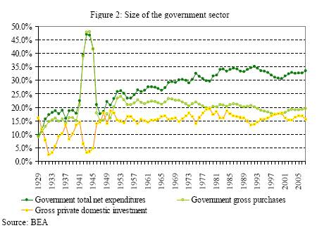
The Fed chairman Ben Bernanke in his recent op-ed piece argued that “given the current economic conditions, banks have generally held their reserves as balances at the Fed.” This is not surprising since, in uncertain times, banks’ liquidity preference rise sharply which reflects on their desire to increase their holdings of liquid assets, such as reserve balances, on their balance sheets.

However, Bernanke pointed out that “as the economy recovers, banks should find more opportunities to lend out their reserves.” The reasoning behind this argument is the so-called multiple deposit creation in which the simple deposit multiplier relates an increase in reserves to an increase in deposits (Bill Mitchell explains it in more details here and here). This is a misconception about banking lending. It presupposes that given an increase in reserve balances (RBs) and excess reserves, assuming that banks do not want hold any excess reserves (ERs), the multiple increase in deposits generated from an increase in the banking system’s reserves can be calculated by the so-called simple deposit multiplier m = 1/rrr, where rrr is the reserve requirement ratio (let’s say 10%). It tells us how much the money supply (M) changes for a given change in the monetary base (B) i.e. M=mB. In this case, the causality runs from the right-hand side of the equation to the left-hand side. The central bank, through open market operations, increases reserve balances leading to an increase in excess reserves in which banks can benefit by extending new loans: ↑RBs → ↑ER → ↑Loans and ↑Deposits.
However, in the real world, money is endogenously created. Banks do not passively await funds to issue loans. Banks extend loans to creditworthy borrowers to meet the needs of trade. In this process, loans create deposits and deposits create reserves. We can illustrate this using T-account as follows:

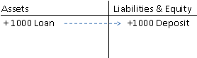
The bank makes a new loan (+1000) and at the same time the borrower’s account is credited with a deposit of an equivalent amount of the loan. Thus, “the increase in the money supply is a consequence of increased loan expenditure, not the cause of it.” (Kaldor and Trevithick, 1981: 5)
In order to meet reserve requirements, banks can obtain reserves in secondary markets or they can borrow from Fed via the discount window.

As noted by Kaldor (1985), Minsky (1975), Goodhart (1984), Moore (1988), Wray (1990), Lavoie (1984) to name a few, money is endogenously created. The supply of money responds to changes in the demand for money. Loans create deposits and deposits create reserves as explained here and here. It turns the deposit multiplier on its head. Goodhart (1994) observed that “[a]lmost all those who have worked in a [central bank] believe that [deposit multiplier] view is totally mistaken; in particular, it ignores the implications of several of the crucial institutional features of a modern commercial banking system….’ (Goodhart, 1994:1424).
As Fulwiller put it, “deposit outflows, if they exceed the bank’s RBs, result in overdrafts. Banks clear this via lowest cost available in money markets or from the Fed.” In this case, let us assume that the bank issues some other liability, such as CDs, in order to obtain the 1000 reserves needed for clearing its overdraft at the Fed.

It reverses the orthodox story of the deposit multiplier (M=mB). Banks are accepting the liability of the borrower and they are creating their own liability, which is the demand deposit. In this process, banks create money by issuing its own liability, which is counted as a component of the money supply. Banks do not wait for the appropriate amount of liquid resources to exist to provide new loans to the public. Instead, as Lavoie (1984) noted ‘money is created as a by-product of the loans provided by the banking system’. Wray (1990) puts it best:
“From the bank’s point of view, money demand is indicated by the willingness of the firm to issue an IOU, and money supply is determined by the willingness of the bank to hold an IOU and issue its own liabilities to finance the purchase of the firm’s IOU…the money supply increases only because two parties willingly enter into commitments.” (Wray 1990 P.74)

As showed above, when banks, overall, are in need of more high-powered money (HPM), they can increase their borrowings with the central bank at the discount rate. Reserve requirements (RRs) cannot be used to control the money supply. In fact, RRs increase the cost of the loans granted by banks. As Wray pointed out “in order to hit the overnight rate target, the central bank must accommodate the demand for reserves—draining the excess or supplying reserves when the system is short. Thus, the supply of reserves is best characterized as horizontal, at the central bank’s target rate.” The central bank cannot control even HPM!The latter is provided through government spending (or Fed lending). The central bank can only modify its discount rate or its rate of intervention on the open market.

Bernanke is concerned that the sharp increase in reserve balances “would produce faster growth in broad money (for example, M1 or M2) and easier credit conditions, which could ultimately result in inflationary pressures.” He is considering the money-price relationship given by the old-fashioned basic quantity theory of money relating prices to the quantity of money based on the equation of exchange (The idea that money is related to price levels and inflation it is not a new idea at all, you can find that, for example, in Hume and other classical economists):

M*V = PQ, where M stands for the money supply (which in the neoclassical model is taken as given, i.e. exogenously determined by monetary policy changes in M), Q is the level of output predetermined at its full employment value by the production function and the operation of a competitive labor market; P is the overall price level and V is the average number of times each dollar is used in transactions during the period. Causality runs from the left-hand side to the right-hand side (nominal output)

According to the monetarist view, under given assumptions, changes in M cause changes in P, i.e. the rate of growth of the money supply (such as M1 and M2) determines the rate of change of the price level. Hence, to avoid high inflations monetary policy should pursue a stable low growth rate in the money supply. The Fed, under Paul Volcker, adopted money targets in October 1979. This resulted in extremely high interest rates, the fed-funds rate was above 20%, the US had double digit unemployment and suffered a deep recession. In addition, the Fed did not hit its money targets. The recession was extremely severe and in 1982 Volker announced that they were abandoning the monetarist experiment. The rate of money growth exploded to as high as 16% p.y, over 5 times what Friedman had recommended, and inflation actually fell (see figure below).

Source: Benjamin Friedman, 1988 :55

The Collapse of the Money-Income and Money-Price Relationships

A closer look at the 1980s and 1990s help us understand the relationship between monetary aggregates such as M1 and M2 and inflation. This is a relationship that did not hold up either in the 1980s nor in the 1990s. As Benjamin Friedman (1988) observed “[a]nyone who had relied on prior credit-based relationships to predict the behavior of income or prices during this period would have made forecasts just as incorrect as those derived from money-based relationships.” (Benjamin Friedman, 1988:63)

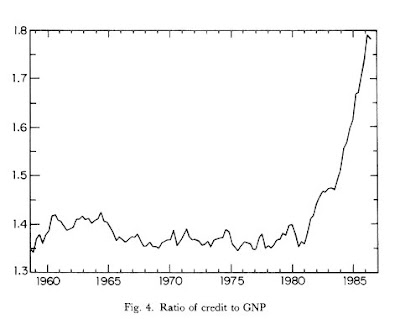
Despite the collapse of the relationship between monetary aggregates and inflation Bernanke still believes that “we must either eliminate these large reserve balances or, if they remain, neutralize any potential undesired effects on the economy.” He noted that “we will need to tighten monetary policy to prevent the emergence of an inflation problem down the road” However, is inflation always and everywhere a monetary phenomenon? The answer is no. The picture below plots the credit-to-GNP ratio. Note that even “the movement of credit during the post-1982 period bore no more relation to income or prices than did that of any of the monetary aggregates.” (Benjamin Friedman, 1988:63, emphasis added)

What about the other monetary aggregates? Benjamin Friedman (1988) pointed out that “[t]he breakdown of long-standing relationships to income and prices has not been confined to the M1 money measure. Neither M2 nor M3, nor the monetary base, nor the total debt of domestic nonfinancial borrowers has displayed a consistent relation- ship to nominal income growth or to inflation during this period.” (ibid, p.62)

Even Mankiw admitted that “[t]he standard deviation of M2 growth was not unusually low during the 1990s, and the standard deviation of M1 growth was the highest of the past four decades. In other words, while the nation was enjoying macroeconomic tranquility, the money supply was exhibiting high volatility. The data give no support for the monetarist view that stability in the monetary aggregates is a prerequisite for economic stability.” Mankiw, 2001: 33)

He concluded that “[i]n February 1993, Fed chairman Alan Greenspan announced that the Fed would pay less attention to the monetary aggregates than it had in the past. The aggregates, he said, ‘do not appear to be giving reliable indications of economic developments and price pressures’… [during the 1990s] increased stability in monetary aggregates played no role in the improved macroeconomic performance of this era.” (Mankiw 2001, 34)

A recent study conducted by the FRBSF also concluded that “there is no predictive power to monetary aggregates when forecasting inflation.” What about the Japanese experience? As the figure below shows, the monetary base exploded but prices actually fell!
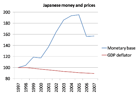
Source: Krugman

What about the US in the 1930s? The same pattern happened, HPM rose sharply and prices were stable!

Source: Krugman

Chairman Bernanke should learn the basic lesson that money is endogenously created. Money comes into the economy endogenously to meet the needs of trade. Most of the money is privately created in private debt contracts. As production and economic activity expand, money expands. The privately created money is used to transfer purchasing power from the future to the present; buy now, pay latter. It allows people to spend beyond what they could spend out of their income or assets they already have. Money is destroyed when debts are repaid.
Consumer price inflation pressures can be caused by struggles over the distribution of income, increasing costs such as labor costs and raw material costs, increasing profit mark-ups, market power, price indexation, imported inflation and so on. As explained above, monetary aggregates are not useful guides for monetary policy.

Another Great Depression?

By Felipe Rezende

In a previous post, I explained that automatic stabilizers- i.e. the fact that the federal government’s budget moves counter-cyclically and in an automatic fashion – imparts a great stabilizing force to aggregate demand.
However, the picture below shows that, during the Great Depression the government sector was too small relatively to the rest of the economy.

Source: Tymoigne, 2008: 12

The implementation of New Deal policies created automatic stabilizers which work by putting a floor under aggregate demand, preventing a deflationary spiral, but they also put ceilings in place, as rapid economic growth translates into rising tax revenues which destroy income and temper the expansion.
Nowadays, the size of the government and the impact of large automatic stabilizers explain why we can have a deep recession but another Great Depression is unlikely.
But how do automatic stabilizers work? What happens over the cycle? Hyman Minsky sheds light on these issues.

Minsky’s financial instability hypothesis can be described as follows. Let us consider that the whole U.S. economy is in a hedge position, i.e. that cash inflows are greater than outflows for every period, so that debt/payment commitments can be fulfilled while safety margin are kept at some positive level, for instance 20%. As firms and households become more optimistic about future earnings, and as their expectations get validated by economy growth, they change their behavior and reduce their margins of safety, let’s say now to 10%.

As the economy booms, and future earnings turn out to be more than expected, firms and households revise their expectations upwards, they begin to believe they were too pessimistic in the past and, therefore, reduce their cushions of safety, and start to take on more and more riskier projects. They have voluntarily moved into a position Minsky called speculative. A speculative position is one in which cash inflows are enough to meet interest payments, i.e. as they cannot repay the principal they need to refinance the outstanding debt. Borrowers start to discount risk and lenders, now more optimistic about prospective future earnings and profits, increase their willingness to lend.

It is now important to introduce how the level of investment is determined according to Minsky’s framework. Firms invest if the demand price of capital exceeds the supply price of current output. “The quantity of investment goods purchased (OId) is determined where PId = PIs” (Tymoigne and Wray 2008, p.9)

The demand price, Pk, is the price that firms are willing to pay for the capital asset. The demand price depends upon the cash flows that ownership is expected to yield and the liquidity of the asset. The curve is horizontal up to the point where firms only commit their internal funds. However, once firms rely on external financing then the subjective borrower’s risk comes into play. This risk is incurred by firms as they may not be able to service their debt. Thus, the price that firms are willing to pay for capital assets decline as the amount they have to borrow to finance it increases.

The supply price, Pi, is the price that firms actually have to pay for the capital good. Firms can use their internal funds up to Oif , and only up to this point, the supply price equals costs + markup. When firms have to borrow to buy capital goods, the supply price of investment is raised by the interest payments on the loan. The curve slopes up after the point Oif because of the lender’s risk. The lender’s risk is the risk the firm will not repay the loan. The more the individual firm borrows, the greater the lender’s risk associated and the higher the interest rate charged on the loan.

When lenders and borrowers become more optimistic about future earnings and profits, they start to discount risks. Firms take on riskier projects and financial institutions riskier loans. Thus, the belief is now that future income will be enough to cover debt commitments. They are in a speculative position.

If there is a change in the economic environment firms’ financial positions may be adversely impacted. Let’s consider the following situation where the economy accelerates and inflation becomes a concern to the monetary authority. The turning point would happen when the Fed decides to increase the overnight interest rate. If the interest rate specified on contracts is allowed to fluctuate, firms incur in higher financial costs to service the loan. At the new circumstance, firms can either abandon the project, as it is no longer profitable at higher interest rates, or they can borrow, from willing financial institutions, the funds they need to meet the interest payments on the previous loans. In other words, if interest rates are increased to such a point where firms’ income inflows are no longer sufficient to meet the firms’ outflows, they have involuntarily moved into a new financial position that Minksy called Ponzi. In a Ponzi scheme, firms have to capitalize interest. If financial institutions become worried about the future performance of the economy as a whole or the firm in particular, and decide to no longer extend those Ponzi loans, then firms are no longer capable of meeting their financial commitments and may default on their loans. This situation can be compounded as firms decide to sell their assets at fire sale prices in order to meet their obligations, setting in a Fisher-type debt deflation process which triggers a domino effect on the economy.

Another situation we could consider as a turning point is one in which firms’ expectations about future earnings/profits is not fulfilled. In such an environment, firms will revise their expectations downwards and cut investment. As we know, this will have a multiplier effect in the economy. As income is reduced, so is consumption. Firms cut back production and investment, which depresses incomes further. The economic activity spirals down squeezing incomes even more. As firms’ income inflows were significantly reduced, firms may get to a point where they can no longer meet their liability commitments. Once again, a debt-deflation process may be set in place by the new economic environment when firms decide to sell their assets at fire sale prices trying to meet their obligations.

Now, we may ask ourselves: what is the role of automatic stabilizers in this process?
The answer becomes even clearer. With big government automatic stabilizers are large enough to offset the swings in private spending. As explained in a previous post, when the economy goes into recession, unemployment rises which means that income transfers such as unemployment compensation and welfare are automatically increased.

According to Minsky, there are 3 major effects derived from automatic stabilizers: the income and employment effect, the cash flow effect, and the portfolio effect. Let me briefly explain each one:

The income effect is the traditional Keynesian multiplier. As the economy slows down, the government deficit increases as there is an automatic increase in spending and a reduction of the amount of taxes collected. As noted in previous posts (here and here), a sovereign government spends by crediting bank accounts which means that the banking system, all else equal, now has excess reserves (ERs). The ERs put a downward pressure on the fed funds rate. If the Fed is to hit its overnight nominal interest rate target, it has to intervene and conduct open market sales (OMS) to drain the ERs. As the Fed provides an interest bearing alternative – such as government securities – this is adds to the private sector’s income.
Therefore, transfer payments and interest payments automatically increase when the economy is moving into a recession.

The other one is the cash flow effect. The idea is that government deficits maintain the flow of profits. Following Kalecki (1972) and national accounting identities, in the simplest version, aggregate profits equal investment plus the government’s deficit, Π = Invest. + Gov. Deficit. In the expanded model, gross profits, after corporate tax, equals investment plus government fiscal deficit plus consumption out of profits plus net exports less saving out of wages, i.e. Π = Invest. + Gov. Deficit + CC + NX– SW. This means that government deficits add to profits (private wealth). The flow of profits prevents the collapse of expectations and the deterioration of private sector’s balance sheet.

Finally, the portfolio effect is generated by the increase in the sale of government bonds as a consequence of the (mostly automatic) increased government deficit (as I have just explained). These bonds are safe assets and their holdings on private sector’s balance sheets help to keep expectations from collapsing below a certain level.

The Big Bank (the Fed) act as a lender of last resort, it can prevent or minimize the fall in asset prices. In other words, the Fed can always put a floor to asset prices. This can be done in many ways, such as by calling up banks and say that they need to lend to investors who want to buy assets. The Fed can also decide to buy a wide range of private assets to smooth market transactions. If the Fed decides to buy a wide range of assets to provide liquidity to markets it smoothes liquidity concerns of market participants. It can also regulate markets and discourage bad loans such as subprime real state booms in some regions so that banks will not provide those loans. However, ceilings should also be put in place such as supervision and regulation, as has been emphasized by William K. Black.

In the current recession, the forecast is that the personal saving rate will reach something like 10% in 2009 and that it could jump to 14-16% by 2010. To meet the private sector rising saving desire the government should implement another stimulus package (in the context of the Krugman’s cross described here, this would be equivalent to a shift of the government sector balance -GSB- curve to the right) thus preventing a deflationary spiral and further declines of income due to rising private sector saving desire. At the same time, it becomes important to adopt policies that make the curve steeper by enhancing the role of automatic stabilizers. One possibility is an employer of last resort program in which the federal government provides a job to everyone willing and able to work at a given nominal wage. As argued in previous posts(here and here) such program would reduce both unemployment and poverty and minimize declines in the economic activity by enhancing the ceilings and floors of the system.

A note on Automatic Stabilizers

What has so far prevented a deep depression in 2009? The answer, as Paul Krugman explained yesterday, are automatic stabilizers. Indeed, as Hyman Minsky emphasized more than 20 years ago in his book Stabilizing an Unstable Economy (1986), this feature of the federal government’s budget – i.e. the fact that it moves counter-cyclically in an automatic fashion – imparts a great stabilizing force to aggregate demand.

The figure below sheds light on the non-discretionary (i.e. automatic) nature of government deficits. In an economic downturn, tax receipts automatically fall, and government expenditures automatically rise, resulting, automatically, in budget deficits. (net govt saving = right hand scale)

Source: Bureau of Economic Analysis (BEA)

The components of government spending that rise automatically are called ‘transfer payments’, that include unemployment compensation, Medicaid, grants-in-aid to state and local government, etc.
With these forms of payment increasing and tax receipts declining due to falling economic activity, the federal budget moves automatically into deficit.

Source: Bureau of Economic Analysis (BEA)

So far the stimulus package was not what saved the US economy. The budget projections show that 24% of the total cost of the stimulus package will occur in fiscal year 2009 (which means $198 billion) and 47% of it occurring in fiscal year 2010.

“The ARRA is estimated in the budget to cost $825.4 billion over the next 10 years. These costs are split between $600.0 billion in increased outlays and $225.4 billion in reduced receipts. Although the cost of the ARRA is spread over 10 years, the budget projections show 24 percent of the total cost occurring in fiscal year 2009 and 47 percent of the total cost occurring in fiscal year 2010…The budget estimates that receipts will be reduced $77.4 billion in fiscal year 2009 and $152.3 billion in fiscal year 2010 primarily because of the tax provisions of ARRA… The budget estimates that outlays will be increased about $120.2 billion for fiscal year 2009 and $237.8 billion for fiscal year 2010 because of the spending and investment provisions of the ARRA.”

As noted in previous posts (here, here, and here), government deficits, themselves, perform an important stabilizing function, because they allow the private sector to net save. Given that during a recession there is a sharp increase in uncertainty and insecurity, the private sector desires to spend less than its income which translates into a rising personal saving rate. In the current recession, the forecast is that the personal saving rate will reach 10% in 2009 and that jump to 14-16% by 2010. Such large decline in consumption means falling sales, production and further declines in GDP. As noted above, to meet the private sector rising saving desire the government should run bigger deficits to prevent a deflationary spiral.

Source: Jan Hatzius, Goldman Sachs

As Minsky emphasized, the problem, during the Great Depression, was that the government sector was too small relative to the rest of the economy; it couldn’t fill the demand gap and allow the private sector to save as much as it desired. In the absence of large enough automatic stabilizers to offset swings in private spending, GDP contracted to the point where desired net nominal saving equaled actual net nominal saving. Note that in second half of the last century, given the private sector’s desire to have positive net nominal saving, the US government normally ran budget deficits.

As Wray pointed out, “Since WWII we have had the longest depression-free period in the nation’s history. However, we have had nine recessions, each of which was preceded by a reduction of deficits relative to GDP.” This directly results from the impact of large swings in the federal government’s budget.

Automatic stabilizers work by putting a floor under aggregate demand, preventing a deflationary spiral, but they also put ceilings in place, as rapid economic growth translates into rising tax revenues which destroy income and temper the expansion. The impact of large automatic stabilizers explains why we can have a deep recession but not a Great Depression. As Wray noted:

“With one brief exception, the federal government has been in debt every year since 1776. In January 1835, for the first and only time in U.S. history, the public debt was retired, and a budget surplus was maintained for the next two years in order to accumulate what Treasury Secretary Levi Woodbury called “a fund to meet future deficits.” In 1837 the economy collapsed into a deep depression that drove the budget into deficit, and the federal government has been in debt ever since. Since 1776 there have been six periods of substantial budget surpluses and significant reduction of the debt. From 1817 to 1821 the national debt fell by 29 percent; from 1823 to 1836 it was eliminated (Jackson’s efforts); from 1852 to 1857 it fell by 59 percent, from 1867 to 1873 by 27 percent, from 1880 to 1893 by more than 50 percent, and from 1920 to 1930 by about a third. (Thayer 1996) The United States has also experienced six periods of depression. The depressions began in 1819, 1837, 1857, 1873, 1893, and 1929. Every significant reduction of the outstanding debt has been followed by a depression, and every depression has been preceded by significant debt reduction. Further, every budget surplus has been followed, usually sooner rather than later, by renewed deficits. However, correlation—even where perfect—never proves causation. Is there any reason to suspect that government surpluses are harmful?”

The Congressional Budget Office’s long-term budget outlook

by Felipe Rezende and Stephanie Kelton

The Congressional Budget Office (CBO) has just released its long-term budget outlook. The dismal report warns:

“Although great uncertainty surrounds long-term fiscal projections, rising costs for health care and the aging of the U.S. population will cause federal spending to increase rapidly under any plausible scenario.” Given these large increases in projected spending, the report went on to caution that “[u]nless tax revenues increase just as rapidly, the rise in spending will produce growing budget deficits and accumulating debt.” Finally, the report asserts that the ensuing “[l]arge budget deficits would reduce national saving, leading to more borrowing from abroad and less domestic investment, which in turn would depress income growth in the United States.”
Once again, we find it necessary to point out the flawed logic of those who certainly ought to have a better understanding of things. First, taxes do not pay for government spending. It would help a great deal if those at the CBO (and elsewhere) would work through the balance sheet entries to decipher exactly how government “financing” operations work.

As Kelton and Wray have explained in earlier posts, the federal government spends by crediting bank accounts. Period. Tax payments to the government result in the destruction of money — high-powered money to be exact — as the banking system clears the checks and reserve accounts are debited. In other words, taxes don’t provide the government with “money to spend”. Tax payments destroy money. Not in theory. Not by assumption. By definition.

Second, growing budget deficits do not reduce national savings. They do just the opposite. Indeed, the private sector — households and firms taken as a whole — cannot attain a surplus position unless some other sector (the public sector or the foreign sector) takes the opposite position. Again, it is an indisputable feature of balance sheet accounting that is governed by the following identity:

Private Sector Surplus = Public Sector Deficit + Current Account Surplus

This fundamental accounting identity can be found in any decent International Economics texbook (see, e.g., Krugman and Obstfeld), and it is one of the most important macroeconomic concepts we can think of. It demonstrates the conditions under which national savings will be positive. Not in theory. Not by assumption. By definition.

Source: Levy Institute

To appreciate the interplay, consider the main sector balances in 2004. The public sector’s deficit of about 5% of GDP was just enough to offset the 5% current account deficit, leaving the private sector with no addition to its net saving (i.e. private sector savings were zero). Today, in contrast, private savings are up sharply because: (1) the public deficit is up sharply and (2) the external deficit is declining. Add today’s (rising) public deficit to today’s (falling) current account deficit and, voila, the CBO’s much-feared explosion in the government deficit has translated into an explosion in private savings.

As for the relationship between savings and investment . . . let’s tackle that accounting lesson next week.

Update: See some Wynne Godley’s pieces here, here , and here. See also Krugman’s piece here.

The Financial Instability Hypothesis

Janet Yellen, President of the San Francisco Federal Reserve, pointed out at the 18th annual conference honoring the work of Hyman P. Minsky that:
“… with the financial world in turmoil, Minsky’s work has become required reading. It is getting the recognition it richly deserves.”

Paul Krugman has also been re-reading Hyman Minsky’s most famous book Stabilizing an Unstable Economy.

Central to Minsky’s view of how financial meltdowns occur is his Financial Instability Hypothesis (FIH) — what has come to be known as ‘an investment theory of the business cycle and a financial theory of investment’. But, what is it all about? Quoting from Minsky . . .

“The theoretical argument of the financial instability hypothesis starts from the characterization of the economy as a capitalist economy with expensive capital assets and a complex, sophisticated financial system… The focus is on an accumulating capitalist economy that moves through real calendar time…”

“The capital development of a capitalist economy is accompanied by exchanges of present money for future money. The present money pays for resources that go into the production of investment output, whereas the future money is the “profits” which will accrue to the capital asset owning firms (as the capital assets are used in production). As a result of the process by which investment is financed, the control over items in the capital stock by producing units is financed by liabilities–these are commitments to pay money at dates specified or as conditions arise. For each economic unit, the liabilities on its balance sheet determine a time series of prior payment commitments, even as the assets generate a time series of conjectured cash receipts…
A part of the financing of the economy can be structured as dated payment commitments in which banks are the central player…”

“Thus, in a capitalist economy the past, the present, and the future are linked not only by capital assets and labor force characteristics but also by financial relations. The key financial relationships link the creation and the ownership of capital assets to the structure of financial relations and changes in this structure…”

“In spite of the greater complexity of financial relations, the key determinant of system behavior remains the level of profits. The financial instability hypothesis incorporates the Kalecki (1965)-Levy (1983) view of profits, in which the structure of aggregate demand determines profits. In the skeletal model, with highly simplified consumption behavior by receivers of profit incomes and wages, in each period aggregate profits equal aggregate investment…”

“In a more complex (though still highly abstract) structure, aggregate profits equal aggregate investment plus the government deficit. Expectations of profits depend upon investment in the future, and realized profits are determined by investment: thus, whether or not liabilities are validated depends upon investment. Investment takes place now because businessmen and their bankers expect investment to take place in the future…”

“The financial instability hypothesis, therefore, is a theory of the impact of debt on system behavior and also incorporates the manner in which debt is validated….”

“The financial instability hypothesis takes banking seriously as a profit-seeking activity. Banks seek profits by financing activity and bankers. Like all entrepreneurs in a capitalist economy, bankers are aware that innovation assures profits. Thus, bankers (using the term generically for all intermediaries in finance), whether they be brokers or dealers, are merchants of debt who strive to innovate in the assets they acquire and the liabilities they market…”

“Three distinct income-debt relations for economic units, which are labeled as hedge, speculative, and Ponzi finance, can be identified.
Hedge financing units are those which can fulfill all of their contractual payment obligations by their cash flows.
Speculative finance units are units that can meet their payment commitments on “income account” on their liabilities, even as they cannot repay the principle out of income cash flows. Such units need to “roll over” their liabilities: (e.g. issue new debt to meet commitments on maturing debt)
For Ponzi units, the cash flows from operations are not sufficient to fulfill either the repayment of principle or the interest due on outstanding debts by their cash flows from operations. Such units can sell assets or borrow. Borrowing to pay interest or selling assets to pay interest (and even dividends) on common stock lowers the equity of a unit, even as it increases liabilities and the prior commitment of future incomes. A unit that Ponzi finances lowers the margin of safety that it offers the holders of its debts.”
“Over periods of prolonged prosperity, the economy transits from financial relations that make for a stable system to financial relations that make for an unstable system.
In particular, over a protracted period of good times, capitalist economies tend to move from a financial structure dominated by hedge finance units to a structure in which there is large weight to units engaged in speculative and Ponzi finance.”
“Furthermore, if an economy with a sizeable body of speculative financial units is in an inflationary state, and the authorities attempt to exorcise inflation by monetary constraint, then speculative units will become Ponzi units and the net worth of previously Ponzi units will quickly evaporate. Consequently, units with cash flow shortfalls will be forced to try to make position by selling out position. This is likely to lead to a collapse of asset values.”
“The financial instability hypothesis is a model of a capitalist economy which does not rely upon exogenous shocks to generate business cycles of varying severity. The hypothesis holds that business cycles of history are compounded out of (i) the internal dynamics of capitalist economies, and (ii) the system of interventions and regulations that are designed to keep the economy operating within reasonable bounds.”

Source: Excerpts from Hyman Minsky’s 1992 paper linked to above.

Update: A good summary of Minsky’s view can be found here and here.