Category Archives: Monetary policy

The Federal Reserve: History, Procedures and Policy

Posted on August 13, 2009 by admin | 2 comments

History of the Fed

The Federal Reserve Act of 1913 created the Fed ‘to furnish an elastic currency, to afford the means of rediscounting commercial paper, to establish a more effective supervision of banking in the United States, and for other purposes’. For many years, the guiding principle of the Fed was the ‘Real Bills Doctrine’ under which the Fed ‘rediscounted’ eligible paper (lending reserves to banks) to facilitate trade. During WWI, the Fed purchased Treasury debt as interest-earning assets, although it was not noticed until the 1920s that this added bank reserves, supporting a multiple expansion of deposits–the ‘deposit multiplier’. In 1924 the Fed first attempted to operate countercyclically, loosening policy in recession to increase bank lending. However, bond purchases did not increase reserves because banks retired loans at the discount window–the first of many times that the Fed learned it could not ‘push on a string’: reserves, loans, and the money supply are demand determined and cannot be increased directly through monetary policy. Symmetrically, analysts found that bond sales merely forced banks to the discount window to replace lost reserves. Hence, the Fed could not control bank lending through attempts to control reserves.

Interpretations of the Fed’s policy during the 1930s range from the Monetarist claim that the Fed reduced the money supply, causing the financial crisis and Great Depression, to the more common belief that the Fed’s inaction made things worse. Actually, the Fed intervened immediately, buying $125 million of Treasury securities on the day of the stock market crash– nearly doubling Fed holdings in one day. The New York Fed also opened its discount window to New York banks that were helping correspondent banks. During the early months of the crisis, the Fed continued to meet currency demand and used open market operations to stabilize interest rates. However, by autumn 1931 gold outflows increased, leading the Fed to raise discount rates to protect gold reserves. The money supply (and reserves) was shrinking not because of Fed policy, but because banks could not find worthy borrowers. In truth, there was little that monetary policy could do; recovery would require fiscal stimulus, which finally came with the New Deal and WWII.

WWII generated huge fiscal deficits, and the Fed agreed in 1942 to peg the Treasury bill rate at 3/8 of 1 per cent. The long-term legacy was a large debt stock, enabling the Fed to use bond purchases rather than discount window borrowing to provide reserves. After the war, the Fed was concerned with potential inflation. In 1947 the Treasury agreed to loosen reins on the Fed, which promptly raised interest rates. The Fed continued to lobby for greater freedom to pursue activist monetary policy, resulting in the 1951 Accord, which abandoned the commitment to maintain low government interest costs. Although not announced explicitly, the Fed clearly targeted interest rates for the next three decades to implement countercyclical policy.

In October 1979, Chairman Paul Volcker, announced a major change: the Fed would use the growth rate of M1 as its target, abandoning interest rates. In practice, the Fed calculated total reserves consistent with its money target, then subtracted borrowed reserves to obtain a non-borrowed reserve target to control money growth. However, if the Fed did not provide sufficient non-borrowed reserves, banks would simply turn to the discount window, causing borrowed reserves to rise (and, in turn, cause the Fed to miss its total reserve target). Because required reserves are always calculated with a lag, the Fed could not refuse to provide needed reserves at the discount window. Thus the Fed found reserves could not be controlled. Further, the rate of growth of M1 actually exploded beyond targets in spite of persistently tight monetary policy, demonstrating the Fed could not hit money targets, either. The attempt to target reserves effectively ended in 1982 (after a very deep recession); the attempt to hit M1 growth targets was abandoned in 1986; and the attempt to target growth of broader money aggregates finally came to an official end in 1993.

Current Policy

Since the early 1990s, the Fed has formulated a new operating procedure that is loosely based on the new monetary consensus—the orthodox approach to monetary theory and policy. The Fed’s policy today is based on five key principles:

1. transparency;
2 gradualism;
3. activism;
4. inflation as the only official goal, but the Fed actually targets distribution;
5. neutral rate as the policy instrument to achieve these goals.

Briefly, over the past decade the Fed has increased “transparency”, telegraphing its moves well in advance and announcing interest rate targets. It also follows a course of gradualism–small adjustments of interest rates (usually 25 to 50 basis points) over several years to achieve ultimate targets. Ironically, by telegraphing its intentions long in advance, and by using a series of small interest rate adjustments, the Fed creates expectations of continued rate hikes (or declines) that it feels compelled to make—for otherwise it can jolt markets—even if economic circumstances change.

These developments have occurred during a long-term trend toward policy activism, contrasting markedly with Milton Friedman’s famous call for rules rather than discretion. The policy instrument used by the Fed is something called a “neutral rate” that varies across countries and through time—an interest rate that is supposed to be consistent with stable GDP growth at full capacity. The neutral rate cannot be recognized until achieved, so it cannot be announced in advance—which is somewhat in conflict with the adoption of transparency. In consequence, the Fed must frequently and actively adjust the fed funds rate hoping to find the neutral rate. But, as Friedman long ago warned, an activist policy has just as much chance of destabilizing the economy as it does to stabilize the economy—matters are made worse when activist policy is guided by invisible neutral rates and fickle market expectations that are fueled by the Fed’s own public musings.

Finally, the Fed claims that its chief concern is inflation. Actually the Fed does target asset prices and income shares, and it shows a strong bias against labor and wages. It will allow strong economic growth and even rising prices, so long as employment remains sluggish and wages do not rise. When, however, the Fed fears that wages might rise, it raises interest rates. Further, there is evidence from transcripts of secret Fed deliberations that it does pay attention to asset prices. Indeed, one of the reasons for rate hikes in 1994 was a desire to “prick” the equity market’s “bubble”. It is probable that rate hikes at the beginning of 2000 were designed to slow the growth of stock prices; and rate hikes that began in 2004 may have been geared to slow real estate speculation.

Chairman Greenspan has been credited with masterful management of monetary policy through the Clinton-era “goldilocks” boom of the 1990s, the recession at the end of the decade, and the economic recovery after 2001. Still, critics note a number of missteps: Greenspan said the stock market was “irrationally exuberant” as early as 1994 (six years before it peaked) and various attempts by the Fed to cool it failed; after stocks crashed in 2000, Greenspan denied it is possible to identify asset price bubbles; the Fed frequently forecast inflationary pressures that never arrived; and sometimes (including summer of 2004) appeared to raise rates when labor markets were weak, while in other cases it seemed to wait too long to lower rates in recession.

Central Banking Today

By their own admission, most central banks now operate with an interest rate target. To hit a non-zero target, the Fed adds or drains reserves to ensure that banks have the amount of reserves desired (or required in nations like the US with official reserve requirements). Reserves are added through discount window loans, purchases of government bonds, and purchases of gold, foreign currencies, or private sector financial assets. To drain reserves, the central bank reverses these actions. It is actually quite easy to determine whether the banking system faces excess or deficient reserves: the overnight rate moves away from target, triggering an offsetting reserve add or drain by the central bank. Central banks also supervise banks and other financial institutions, engage in lender of last resort activities (a bank in financial difficulty may not be able to borrow reserves in the private lending market even if aggregate reserves are sufficient), and occasionally adopt credit controls, usually on a temporary basis. We will ignore these types of activities as of secondary interest.

When the operating procedure is laid bare, it is obvious that views about controlling reserves, or sterilization of international capital flows, or central bank “financing” of treasury deficits by “printing money” are incorrect. If international payments flows or domestic fiscal actions create excess reserves, the central bank has no choice but to drain the excess–or the overnight rate falls toward zero. On the other hand, if international payments flows or domestic fiscal actions leave banks with insufficient reserves, overnight rates rise above target. For this reason, the quantity of reserves is never discretionary.

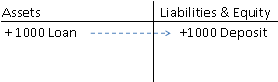
Likewise, the view that a central bank might choose to “print money” to finance a budget deficit is flawed. In practice, modern sovereign governments spend by crediting bank accounts and tax by debiting them. Clearing with the government takes place using reserves, that is, on the accounts of the central bank. Deficits lead to net credits of reserves; if excessive, they are drained through bond sales. These activities are coordinated with the Treasury, which issues new bonds in step (whether before or after is not material) with deficit spending. This is because the central bank would run out of bonds to sell. In countries in which the central bank pays interest on reserves, bond sales are unnecessary because interest-paying reserves serve the same purpose—that is, to ensure the overnight interest rate cannot fall below the target. The important point is that central bank operations are not discretionary, but are required to hit interest rate targets.

In sum, the Fed and other central banks of countries with sovereign currencies have complete policy discretion regarding the overnight interest rate. This does not mean that they do not take into account possible impacts of their target on inflation, unemployment, the trade balance, or the exchange rate. Further, central banks often react to budget deficits by raising the overnight interest rate target. These policy actions are discretionary. But what is not discretionary is the quantity of reserves in a system such as that adopted by the US—where banks do not earn interest on reserves. This is because a shortage causes the interest rate to rise above target; an excess causes it to fall. The Fed is forced to defend its target by intervening—adding or draining reserves. A country like Canada that pays interest on positive reserve holdings (and charges interest on reserve lending) need not drain “excess” reserves—because they are not really excessive. Indeed, there is no real distinction between reserves that pay interest or treasury bills that pay interest—both serve the same purpose of maintaining a positive overnight interest rate, so there is no reason to sell bills to banks to “drain excess reserves” in such countries.

We conclude that central banking policy really boils down to interest rate setting and that calls for controlling reserves or the money supply are misguided. However, it is far from clear that interest rates matter much, especially when transparency and gradualism eliminate the element of surprise. Thus, the view that monetary policy can “fine-tune” the economy is probably in error.

References:

Friedman, Milton. 1969. The Optimal Quantity of Money and Other Essays. Chicago: Aldine.

Wray, L. Randall. Understanding Modern Money: The Key to Full Employment and Price Stability, Edward Elgar Publishing, 1998.

—-. The Fed and the New Monetary Consensus: The Case for Rate Hikes, Part Two Levy Policy Brief No. 80, 2004 December 2004

2 Comments

Posted in L. Randall Wray, Monetary policy, Uncategorized

Tagged Federal Reserve, L. Randall Wray, Monetary policy

How to Implement True, Full Employment

Posted on August 12, 2009 by admin | 5 comments

By L. Randall Wray

We will briefly describe a program that would generate true, full employment, price stability, and currency stability. We will show that this program can be adopted in any nation that issues its own currency. Our presentation consists of three sections. First, we briefly examine a pilot program at the University of Missouri—Kansas City (UMKC). This provides the basis for the analysis in the second section of the functioning of a national monetary system. Finally, we show how this knowledge can be used to construct a public service program (PSE) that guarantees true, full employment with price and currency stability.

The Buckaroo Program

In the United States, there is a growing movement on college campuses to increase student involvement in their communities, particularly through what is known as “service-learning” in which students participate in community service activities organized by local community groups. It should become obvious that a modern monetary economy that adopts the full employment program described here will operate much like our community service hours program.

We have chosen to design our program as a “monetary” system, creating paper notes, “buckaroos” (after the UMKC mascot, a kangaroo), with the inscription “this note represents one hour of community service by a UMKC student”, and denominated as “one roo hour”. Each student is required to pay B25 to the UMKC “Treasury” each semester. Approved community service providers (state and local government offices, university offices, public school districts, and not-for-profit agencies) submit bids for student service hours to the Treasury, which “awards” special drawing rights (SDRs) to the providers so long as basic health, safety, and liability standards are met. The providers then draw on their SDRs as needed pay students B1 per hour worked. This is equivalent to “spending” by the UMKC treasury. Students then pay their taxes with buckaroos, retiring Treasury liabilities.

Several implications are immediately obvious. First, the UMKC treasury cannot collect any buckaroo taxes until it has spent some buckaroos. Second, the Treasury cannot collect more buckaroos in payment of taxes than it has previously spent. This means that the “best” the Treasury can hope for is a “balanced budget”. Actually, it is almost certain that the Treasury will run a deficit as some buckaroos are “lost in the wash” or hoarded for future years. While it is possible that the Treasury could run a surplus in future years, this would be limited by the quantity of previously hoarded buckaroos that could be used to pay taxes. Third, and most important, it should be obvious that the Treasury faces no “financial constraints” on its ability to spend buckaroos. Indeed, the quantity of buckaroos provided is “market demand determined”, by the students who desire to work to obtain buckaroos and by the providers who need student labor. Furthermore, it should be obvious that the Treasury’s spending doesn’t depend on its tax receipts. To drive the point home, we can assume that the Treasury always burns every buckaroo received in payment of taxes. In other words, the Treasury does not impose taxes in order to ensure that buckaroos flow into its coffers, but rather to ensure that student labor flows into community service. More generally, the Treasury’s budget balance or imbalance doesn’t provide any useful information to UMKC regarding the program’s success or failure. A Treasury deficit, surplus, or balance provides useless accounting data.

Note that each student has to obtain a sufficient number of buckaroos to meet her tax liability. Obviously, an individual might choose to earn, say, B35 in one semester, holding B10 as a hoard after paying the B25 tax for that semester. The hoards, of course, are by definition equal to the Treasury’s deficit. UMKC has decided to encourage “thrift” by selling interest-earning buckaroo “bonds”, purchased by students with excess buckaroo hoards. This is usually described as government “borrowing”, thought to be necessitated by government deficits. Note however, that the Treasury does not “need” to borrow its own buckaroos in order to deficit spend—no matter how high the deficit, the Treasury can always issue new buckaroos. Indeed, the Treasury can only “borrow” buckaroos that it has already spent, in fact, that it has “deficit spent”. Finally, note that the Treasury can pay any interest rate it wishes, because it does not “need” to “borrow” from students. For this reason, Treasury bonds should be seen as an “interest rate maintenance account” designed to keep the base rate at the Treasury’s target interest rate. Without such an account, the “natural base interest rate” is zero for buckaroo hoards created through deficit spending. Note that no matter how much the Treasury spends the base rate would never rise above zero unless the Treasury offers positive interest rates; in other words, Treasury deficits do not place any pressure on interest rates.

What determines the value of buckaroos? From the perspective of the student, the “cost” of a buckaroo is the hour of labor that must be provided; from the perspective of the community service provider, a buckaroo buys an hour of student labor. So, on average, the buckaroo is worth an hour of labor—more specifically, an hour of average student labor. Note that we can determine the value of the buckaroo without reference to the quantity of buckaroos issued by the Treasury. Whether the Treasury spends a hundred thousand buckaroos a year, or a million a year, the value is determined by what students must do to obtain them.

The Treasury’s deficit each semester is equal to the “extra” demand for buckaroos coming from students; indeed, it is the “extra” demand that determines the size of the Treasury’s deficit. We might call this “net saving” of buckaroos, and it is equal—by definition—to the Treasury’s deficit over the same period. What if the Treasury decided it did not want to run deficits, and so proposed to limit the total number of buckaroos spent in order to balance the budget? In this case, it is almost certain that some students would be unable to meet their tax liability. Unlucky, procrastinating students would find it impossible to find a community service job, thus would find themselves “unemployed” and would be forced to borrow, beg, or steal buckaroos to meet their tax liabilities. Of course, any objective analysis would find the source of the unemployment in the Treasury’s policy, and not in the characteristics of the unemployed. Unemployment at the aggregate level is caused by insufficient Treasury spending.

Some of thisanalysis applies directly to our economic system as it actually operates, while some of it would apply to the operation of our system if it were to adopt a full employment program. Let us examine the operation of a modern money system.

Modern Monetary Systems

In all modern economies, money is a creature of the State. The State defines money as that which it accepts at public pay offices (mainly, in payment of taxes). Taxes create a demand for money, and government spending provides the supply, just as our buckaroo tax creates a demand for buckaroos, while spending by the Treasury provides the supply. The government does not “need” the public’s money in order to spend; rather, the public needs the government’s money in order to pay taxes. This means that the government can buy whatever is for sale in terms of its money merely by providing it.

Because the public will normally wish to hold some extra money, the government will normally have to spend more than it taxes; in other words, the normal requirement is for a government deficit, just as the UMKC Treasury always runs a deficit. Government deficits do not require “borrowing” by the government (bond sales), rather, the government provides bonds to allow the public to hold interest-bearing alternatives to non-interest-bearing government money. Further, markets cannot dictate to government the interest rate it must pay on its debt, rather, the government determines the interest rate it will pay as an alternative to non-interest-earning government money. This stands conventional analysis on its head: fiscal policy is the primary determinant of the quantity of money issued, while monetary policy primarily has to do with maintaining positive interest rates through bond sales—at the interest rate the government chooses.

In summary, governments issue money to buy what they need; they tax to generate a demand for that money; and then they accept the same money in payment of the tax. If a deficit results, that just lets the population hoard some of the money. If the government wants to, it can let the population trade the money for interest earning bonds, but the government never needs to borrow its own money from the public.

This does not mean that the deficit cannot be too big, that is, inflationary; it can also be too small, that is deflationary. When the deficit is too small, unemployment results (just as it results at UMKC when the Treasury’s spending of buckaroos is too small). The fear, of course, is that government deficits might generate inflation before full employment can be reached. In the next section we describe a proposal that can achieve full employment while actually enhancing price stability.

Public Service Employment and Full Employment with Price and Currency Stability

Very generally, the idea behind our proposal is that the national government provides funding for a program that guarantees a job offer for anyone who is ready, willing and able to work. We call this the Public Service Employment program, or PSE. What is the PSE program? What do we want to get out of it?

1. It should offer a job to anyone who is ready, willing and able to work; regardless of race or gender, regardless of education, regardless of work experience; regardless of immigration status; regardless of the performance of the economy. Just listing those conditions makes it clear why private firms cannot possibly offer an infinitely elastic demand for labor. The government must play a role. At a minimum, the national government must provide the wages and benefits for the program, although this does not actually mean that PSE must be a government-run program.

2. We want PSE to hire off the bottom. It is an employment safety net. We do not want it to compete with the private sector or even with non-PSE employment in the public sector. It is not a program that operates by “priming the pump”, that is, by raising aggregate demand. Trying to get to full employment simply by priming the pump with military spending could generate inflation. That is because military Keynesianism hires off the top. But by definition, PSE hires off the bottom; it is a bufferstock policy—and like any bufferstock program, it must stabilize the price of the bufferstock—in this case, wages at the bottom.

3. We want full employment, but with loose labor markets. This is virtually guaranteed if PSE hires off the bottom. With PSE, labor markets are loose because there is always a pool of labor available to be hired out of PSE and into private firms. Right now, loose labor markets can only be maintained by keeping people out of work—the old reserve army of the unemployed approach.

4. We want the PSE compensation package to provide a decent standard of living even as it helps to maintain wage and price stability. We have suggested that the wage ought to be set at $6.25/hr in the USA to start. A package of benefits could include healthcare, childcare, sick leave, vacations, and contributions to Social Security so that years spent in PSE would count toward retirement.

5. We want PSE experience to prepare workers for post-PSE work—whether in the private sector or in government. Thus, PSE workers should learn useful work habits and skills. Training and retraining will be an important component of every PSE job.

6. Finally, we want PSE workers to do something useful. For the U.S.A. we have proposed that they focus on provision of public services, however, a developing nation may have much greater need for public infrastructure; for roads, public utilities, health services, education. PSE workers should do something useful, but they should not do things that are already being done, and especially should not compete with the private sector.

These six features pretty well determine what a PSE program ought to look like. This still leaves a lot of issues to be examined. Who should administer the program? Who should do the hiring and supervision of workers? Who should decide exactly what workers will do? There are different models consistent with this general framework, and different nations might take different approaches. Elsewhere (Wray 1998, 1999) I have discussed the outlines of a program designed specifically for the USA. Very briefly, I suggest that given political realities in the USA, it is best to decentralize the program as much as possible. State and local governments, school districts, and non-profit organizations would be allowed to hire as many PSE workers as they could supervise. The federal government would provide the basic wage and benefit package, while the hiring agencies would provide supervision and capital required by workers (some federal subsidy of these expenses might be allowed). All created jobs would be expected to increase employability of the PSE workers (by providing training, experience, work records); PSE employers would compete for PSE workers, helping to achieve this goal. No PSE employer would be allowed to use PSE workers to substitute for existing employees (representatives of labor should sit on all administrative boards that make hiring decisions). Payments by the federal government would be made directly to PSE workers (using, for example, Social Security numbers) to reduce potential for fraud.

Note that some countries might choose a much higher level of centralization. In other words, program decentralization is dictated purely by pragmatic and political considerations. The only essential feature is that funding must come from the national government, that is, from the issuer of the currency.

Before concluding, let us quickly address some general questions. First, many people wonder about the cost—can we afford full employment? To answer this, we must distinguish between real costs and financial expenditures. Unemployment has a real cost—the output that is lost when some of the labor force is involuntarily unemployed, the burdens placed on workers who must produce output to be consumed by the unemployed, the suffering of the unemployed, and social ills generated by unemployment and poverty. From this perspective, providing jobs for the unemployed will reduce real costs and generate net real benefits for society. Indeed, it is best to argue that society cannot afford unemployment, rather than to suppose that it cannot afford employment!

On the other hand, most people are probably concerned with the financial cost of full employment, or, more specifically, with the impact on the government’s budget. How will the government pay for the program? It will write checks just as it does for any other program. (See Wray 1998.) This is why it is so important to understand how the modern money system works. Any nation that issues its own currency can financially afford to hire the unemployed. A deficit will result only if the population desires to save in the form of government-issued money. In other words, just as in UMKC’s buckaroo program, the size of the deficit will be “market demand” determined by the population’s desired net saving.

Economists usually fear that providing jobs to people who want to work will cause inflation. Thus, it is necessary to explain how our proposed program will actually contribute to wage stability, promoting price stability. The key is that our program is designed to operate like a “buffer stock” program, in which the buffer stock commodity is sold when there is upward pressure on its price, or bought when there are deflationary pressures. Our proposal is to use labor as the buffer stock commodity, and as is the case with any buffer stock commodity, the program will stabilize the commodity’s price. The government’s spending on the program is based on a “fixed price/floating quantity” model, hence, cannot contribute to inflation.

Note that the government’s spending on the full employment program will fluctuate countercyclically. When the private sector reduces spending, it lays-off workers who then flow into the bufferstock pool, working in the full employment program. This automatically increases total government spending, but not prices because the wage paid is fixed. As the quantity of workers hired at the fixed wage rises, this results in a budget deficit. On the other hand, when the private sector expands, it pulls workers out of the bufferstock pool, shrinking government spending and thus reducing deficits. This is a powerful automatic stabilizer that operates to ensure the government’s spending is at just the right level to maintain full employment without generating inflation.

REFERENCES

Wray, L. Randall. 1998. Understanding Modern Money: the key to full employment and price stability, Cheltenham: Edward Elgar.

—–. 1999. “Public Service Employment—Assured Jobs Program: further considerations“, Journal of Economic Issues, Vol. 33, no. 2, pp. 483-490.

5 Comments

Posted in L. Randall Wray, Monetary policy, Policy and Reform, Taxes, The Federal Government Deficit, The National Debt, Uncategorized, Unemployment

Tagged Fiscal Policy, L. Randall Wray, Monetary policy, Policy and Reform, Taxes, The Federal Government Deficit, The National Debt, unemployment

Another Embarrassing Blunder by Chairman Bernanke

Posted on July 22, 2009 by admin | 9 comments

By Felipe Rezende

The Fed chairman Ben Bernanke in his recent op-ed piece argued that “given the current economic conditions, banks have generally held their reserves as balances at the Fed.” This is not surprising since, in uncertain times, banks’ liquidity preference rise sharply which reflects on their desire to increase their holdings of liquid assets, such as reserve balances, on their balance sheets.

However, Bernanke pointed out that “as the economy recovers, banks should find more opportunities to lend out their reserves.” The reasoning behind this argument is the so-called multiple deposit creation in which the simple deposit multiplier relates an increase in reserves to an increase in deposits (Bill Mitchell explains it in more details here and here). This is a misconception about banking lending. It presupposes that given an increase in reserve balances (RBs) and excess reserves, assuming that banks do not want hold any excess reserves (ERs), the multiple increase in deposits generated from an increase in the banking system’s reserves can be calculated by the so-called simple deposit multiplier m = 1/rrr, where rrr is the reserve requirement ratio (let’s say 10%). It tells us how much the money supply (M) changes for a given change in the monetary base (B) i.e. M=mB. In this case, the causality runs from the right-hand side of the equation to the left-hand side. The central bank, through open market operations, increases reserve balances leading to an increase in excess reserves in which banks can benefit by extending new loans: ↑RBs → ↑ER → ↑Loans and ↑Deposits.
However, in the real world, money is endogenously created. Banks do not passively await funds to issue loans. Banks extend loans to creditworthy borrowers to meet the needs of trade. In this process, loans create deposits and deposits create reserves. We can illustrate this using T-account as follows:

The bank makes a new loan (+1000) and at the same time the borrower’s account is credited with a deposit of an equivalent amount of the loan. Thus, “the increase in the money supply is a consequence of increased loan expenditure, not the cause of it.” (Kaldor and Trevithick, 1981: 5)
In order to meet reserve requirements, banks can obtain reserves in secondary markets or they can borrow from Fed via the discount window.

As noted by Kaldor (1985), Minsky (1975), Goodhart (1984), Moore (1988), Wray (1990), Lavoie (1984) to name a few, money is endogenously created. The supply of money responds to changes in the demand for money. Loans create deposits and deposits create reserves as explained here and here. It turns the deposit multiplier on its head. Goodhart (1994) observed that “[a]lmost all those who have worked in a [central bank] believe that [deposit multiplier] view is totally mistaken; in particular, it ignores the implications of several of the crucial institutional features of a modern commercial banking system….’ (Goodhart, 1994:1424).
As Fulwiller put it, “deposit outflows, if they exceed the bank’s RBs, result in overdrafts. Banks clear this via lowest cost available in money markets or from the Fed.” In this case, let us assume that the bank issues some other liability, such as CDs, in order to obtain the 1000 reserves needed for clearing its overdraft at the Fed.

It reverses the orthodox story of the deposit multiplier (M=mB). Banks are accepting the liability of the borrower and they are creating their own liability, which is the demand deposit. In this process, banks create money by issuing its own liability, which is counted as a component of the money supply. Banks do not wait for the appropriate amount of liquid resources to exist to provide new loans to the public. Instead, as Lavoie (1984) noted ‘money is created as a by-product of the loans provided by the banking system’. Wray (1990) puts it best:
“From the bank’s point of view, money demand is indicated by the willingness of the firm to issue an IOU, and money supply is determined by the willingness of the bank to hold an IOU and issue its own liabilities to finance the purchase of the firm’s IOU…the money supply increases only because two parties willingly enter into commitments.” (Wray 1990 P.74)

As showed above, when banks, overall, are in need of more high-powered money (HPM), they can increase their borrowings with the central bank at the discount rate. Reserve requirements (RRs) cannot be used to control the money supply. In fact, RRs increase the cost of the loans granted by banks. As Wray pointed out “in order to hit the overnight rate target, the central bank must accommodate the demand for reserves—draining the excess or supplying reserves when the system is short. Thus, the supply of reserves is best characterized as horizontal, at the central bank’s target rate.” The central bank cannot control even HPM!The latter is provided through government spending (or Fed lending). The central bank can only modify its discount rate or its rate of intervention on the open market.

Bernanke is concerned that the sharp increase in reserve balances “would produce faster growth in broad money (for example, M1 or M2) and easier credit conditions, which could ultimately result in inflationary pressures.” He is considering the money-price relationship given by the old-fashioned basic quantity theory of money relating prices to the quantity of money based on the equation of exchange (The idea that money is related to price levels and inflation it is not a new idea at all, you can find that, for example, in Hume and other classical economists):

M*V = PQ, where M stands for the money supply (which in the neoclassical model is taken as given, i.e. exogenously determined by monetary policy changes in M), Q is the level of output predetermined at its full employment value by the production function and the operation of a competitive labor market; P is the overall price level and V is the average number of times each dollar is used in transactions during the period. Causality runs from the left-hand side to the right-hand side (nominal output)

According to the monetarist view, under given assumptions, changes in M cause changes in P, i.e. the rate of growth of the money supply (such as M1 and M2) determines the rate of change of the price level. Hence, to avoid high inflations monetary policy should pursue a stable low growth rate in the money supply. The Fed, under Paul Volcker, adopted money targets in October 1979. This resulted in extremely high interest rates, the fed-funds rate was above 20%, the US had double digit unemployment and suffered a deep recession. In addition, the Fed did not hit its money targets. The recession was extremely severe and in 1982 Volker announced that they were abandoning the monetarist experiment. The rate of money growth exploded to as high as 16% p.y, over 5 times what Friedman had recommended, and inflation actually fell (see figure below).

Source: Benjamin Friedman, 1988 :55

The Collapse of the Money-Income and Money-Price Relationships

A closer look at the 1980s and 1990s help us understand the relationship between monetary aggregates such as M1 and M2 and inflation. This is a relationship that did not hold up either in the 1980s nor in the 1990s. As Benjamin Friedman (1988) observed “[a]nyone who had relied on prior credit-based relationships to predict the behavior of income or prices during this period would have made forecasts just as incorrect as those derived from money-based relationships.” (Benjamin Friedman, 1988:63)

Despite the collapse of the relationship between monetary aggregates and inflation Bernanke still believes that “we must either eliminate these large reserve balances or, if they remain, neutralize any potential undesired effects on the economy.” He noted that “we will need to tighten monetary policy to prevent the emergence of an inflation problem down the road” However, is inflation always and everywhere a monetary phenomenon? The answer is no. The picture below plots the credit-to-GNP ratio. Note that even “the movement of credit during the post-1982 period bore no more relation to income or prices than did that of any of the monetary aggregates.” (Benjamin Friedman, 1988:63, emphasis added)

What about the other monetary aggregates? Benjamin Friedman (1988) pointed out that “[t]he breakdown of long-standing relationships to income and prices has not been confined to the M1 money measure. Neither M2 nor M3, nor the monetary base, nor the total debt of domestic nonfinancial borrowers has displayed a consistent relation- ship to nominal income growth or to inflation during this period.” (ibid, p.62)

Even Mankiw admitted that “[t]he standard deviation of M2 growth was not unusually low during the 1990s, and the standard deviation of M1 growth was the highest of the past four decades. In other words, while the nation was enjoying macroeconomic tranquility, the money supply was exhibiting high volatility. The data give no support for the monetarist view that stability in the monetary aggregates is a prerequisite for economic stability.” Mankiw, 2001: 33)

He concluded that “[i]n February 1993, Fed chairman Alan Greenspan announced that the Fed would pay less attention to the monetary aggregates than it had in the past. The aggregates, he said, ‘do not appear to be giving reliable indications of economic developments and price pressures’… [during the 1990s] increased stability in monetary aggregates played no role in the improved macroeconomic performance of this era.” (Mankiw 2001, 34)

A recent study conducted by the FRBSF also concluded that “there is no predictive power to monetary aggregates when forecasting inflation.” What about the Japanese experience? As the figure below shows, the monetary base exploded but prices actually fell!

Source: Krugman

What about the US in the 1930s? The same pattern happened, HPM rose sharply and prices were stable!

Source: Krugman

Chairman Bernanke should learn the basic lesson that money is endogenously created. Money comes into the economy endogenously to meet the needs of trade. Most of the money is privately created in private debt contracts. As production and economic activity expand, money expands. The privately created money is used to transfer purchasing power from the future to the present; buy now, pay latter. It allows people to spend beyond what they could spend out of their income or assets they already have. Money is destroyed when debts are repaid.
Consumer price inflation pressures can be caused by struggles over the distribution of income, increasing costs such as labor costs and raw material costs, increasing profit mark-ups, market power, price indexation, imported inflation and so on. As explained above, monetary aggregates are not useful guides for monetary policy.

9 Comments

Posted in Felipe C. Rezende, Monetary policy, Uncategorized

Tagged Federal Reserve, Felipe C. Rezende, inflation, Monetary policy

Why Negative Nominal Interest Rates Miss the Point, Part II—Understanding the Excess Reserve Tax

Posted on July 14, 2009 by admin | 15 comments

By Scott Fullwiler

My previous post critiquing Scott Sumner’s (and others’) proposal for negative nominal interest rates brought a most welcome response from Prof. Sumner in the comments section. The comments section has a character limit that I’m sure to go over in response to his response, however; hence this post. The core of my reply and critique here is twofold: first, Sumner misunderstands the Fed’s monetary operations, particularly the details of reserve accounting (that is, the dynamics of changes to the Fed’s balance sheet); and second, the proposal assumes the textbook money multiplier when in fact this doesn’t apply to the U.S. or any other nation not operating under a fixed exchange rate policy such as a gold standard or currency board.

Sumner’s original proposal, as he notes in the comments, can be found here. The basics of the proposal are that the Fed would set a modestly negative rate to be paid on bank excess reserves (ERs; he has discussed rates -2% and -4% on his blog); given this penalty, banks would then be encouraged via the monetarist “excess cash balance” mechanism, as he describes it (i.e., the money multiplier) to create deposits that would thereby transform these ERs into required reserves that would not be subject to the penalty. The problem the proposal supposedly solves is that banks are “sitting” on their excess balances (currently around $700 billion) and need an incentive to “move [ERs] into cash in circulation.”

Turning to reserve accounting, consider Sumner’s comment on my original post:”The proposal would not drive interbank loan rates significantly negative, as banks could always exchange ERs for T-bills. And T-bill yields could not go significantly negative because non-bank holders of T-bills can always hold cash.”
As a small aside, I’m puzzled why he would think my critique centered on the interbank rate or T-Bill rate, as my critique was instead directed at the “excess cash balance” mechanism or money multiplier; that these rates might turn negative is not necessarily problematic in my opinion, but that’s what will happen, so I noted as much. But I digress.

Sumner’s statement “banks could always exchange ERs for T-bills” misses an important point . . . namely because this transaction would not extinguish the reserve balances, but rather move them to the (in the case of a non-bank seller) seller’s bank. So, let’s assume that the seller’s bank had no undesired ERs prior to the sale. Now, after the sale, it DOES have undesired ERs (while, yes, the non-bank seller can now hold deposits or CDs or whatever).

The fundamental point here is that ONLY changes to the Fed’s balance sheet can change the aggregate quantity of reserve balances held by banks. In other words, the Fed is the MONOPOLY supplier of net reserve balances to the banking system. This is not an opinion or a theory, but rather a FACT of double-entry reserve accounting . . . aggregate reserve balances are on the liability side of the Fed’s balance sheet, only a change somewhere else on the Fed’s balance sheet can alter them. And the T-bill purchase Sumner describes does not involve the Fed’s balance sheet.

In fact, the only way a T-bill purchase would extinguish reserve balances as Sumner proposes is if the purchase is done at auction (from his quote, clearly not what he was intending), which would in fact be a roundabout way of having the Fed simply add balances to the Treasury’s account (again, I’ll assume he wasn’t intending this with his proposal).

So, if we have an aggregate banking system with some undesired excess balances, the banks individually can trade these among themselves however they want (fed funds market, T-bill transactions, repos, and so forth), but the undesired excess simply moves from bank to bank, never going away. It’s well established in the academic literature on the fed funds market that this brings the fed funds rate down toward the level paid to banks on reserve balances (which Sumner’s wants negative). Hopefully it’s clear, though, that my criticism in this case is not and was not about the fact that the interbank rate would fall, but rather about the inherent misunderstanding of reserve accounting in the proposal (and, alas, in Sumner’s comment above).Very briefly to his point on T-bill rates, any individual bank will purchase T-bills at yields higher than its marginal return on ERs at the Fed. These purchases move those reserves to other member banks, which then do the same, thereby driving T-bill rates down to or even below the Fed funds rate. Furthermore, negative T-bill rates have for technical reasons in fact been a common occurrence in both Japan and the U.S.

For a little more detail, consider Sumner’s following comment from his original proposal: “We also know that banks hold very low levels of ERs any time the opportunity cost (in terms of the T-bill alternative) is even modestly positive. Thus in the summer of 2008 when the target rate was only 2%, ERs were still very low.”
Wrong. Banks DESIRE to hold low levels of ERs when the opportunity cost is even modestly positive. But they will by definition in the aggregate hold as many as the Fed leaves circulating, since the Fed is the monopoly supplier of aggregate reserve balances. Prior to September 2008, the Fed ACCOMMODATED banks’ desire to hold low levels of ERs by draining any additional balances via reverse repos and such—a process that had become very complicated starting in August 2007 (but that’s a long story in itself). Virtually every other central bank does the same under normal circumstances.

After September 2008, circumstances were not normal, as the Fed (in its view, at least) no longer had enough purchased assets to sell or repo to drain any undesired ERs created via its various standing facilities. Consequently, while banks individually actually may have DESIRED to hold lower levels of ERs (though their desired quantity was admittedly increased above normal given substantial concerns about counterparty risks), in the aggregate, they had no choice but to hold a larger quantity (again, though, the Fed’s repeated flubs with instituting payment on reserve balances kept the fed funds rate well below the target and thereby minimized any opportunity cost that might have existed).

I don’t want to dwell on this particular point too much, as it moves a bit too far ahead given that, for Sumner’s proposal, at issue isn’t the aggregate quantity of reserve balances but rather how to transform the ERs to required reserves. But clarity on reserve accounting in monetary operations is absolutely essential, as we’ll see again below.

As for transforming the ERs to required reserves, Sumner writes in his original post that “from a monetarist excess cash balance perspective, the problem is the hoarding of ERs by banks.” So, now quoting from his comments on my post, his excess reserve tax proposal is intended “to move ERs into cash in circulation . . . [as it] . . . relies on the monetarist ‘excess cash balance’ mechanism.” From his original post, “a penalty rate on ERs of say 4% should bring ERs down to extremely low levels.”

That is, penalizing banks for holding ERs is proposed in order to encourage banks to create more deposits, thus raising reserve requirements and lowering the relative quantity of ERs among existing reserve balances.

This is the money multiplier framework, which is inapplicable to the US monetary system, as noted above. So what this errant view does is cause Sumner to get the problem wrong.

To see why, consider a bank with no ERs at all. Suppose a credit worthy customer comes through the door and wants a loan and the bank deems the loan profitable. Does the bank have the operational ability to create the loan? In EVERY country not operating under a fixed exchange rate system such as a gold standard or a currency board, the answer is YES. As I have explained in previous posts (here and here), if the bank ends up short on its reserve requirements, it incurs an overdraft automatically from the Fed at a stated penalty rate as a matter of accounting. In practice, this wouldn’t actually occur for at least 2.5 weeks given lagged reserve accounting in the US, by which time the bank’s liquidity manager would have raised any required funds via any number of sources, but that’s not really the point.

The point is that the reserve requirement can only impose a “cost” penalty on the bank, not constrain it from lending. Further, in the aggregate, central banks act to avoid such additional costs which would cause the interbank rate to trade above the central bank’s target rate by ACCOMMODATING the banking system’s demands for balances to meet reserve requirements before such overdrafts occur. They do this out of necessity since leaving banks in the aggregate short of meeting requirements would mean that deficient banks would bid the interbank rate up as they tried to entice other banks to lend, pushing the rate up above the central bank’s target until it reached the central bank’s stated penalty for a reserve deficiency. At this point, banks would be theoretically indifferent between borrowing from another bank and simply incurring the overdraft at the same rate.

Now consider a bank with substantial ERs. Does it have any more operational ability to create a loan than the bank in the previous example? Certainly not, as the bank in the previous example has NO operational limits to its abilities to lend–it will obtain any necessary reserves from other banks and the central bank will provide more to the aggregate system should that be necessary to achieve its target rate.

The only instance in which the previous bank might change its plans is where a central bank does not accommodate its interest rate target but instead provides the overdraft at a penalty to a deficient bank. But all this would do is raise the interest rate the bank would be willing to lend at (since its own costs would have risen via the penalty). So, again, the bank would not be constrained by reserve availability. It just means that infinite funds would still be available but at a higher interest rate. Again, this has not been the practice of modern central banks (even for the Fed during its so-called “monetarist experiment”).

As an aside, let’s state this another way. That is, a central bank that attempts to target the quantity of aggregate reserve balances such that it forces individual banks to meet reserve requirements via overdrafts at a penalty is NOT targeting directly the quantity of reserve balances but rather setting a de facto target at its stated penalty rate. As Warren Mosler says, central bank operations are ALWAYS about price, not quantity, as a matter of institutional structure.

Now assume that the excess reserve tax is imposed on the bank holding the ERs. Does this make it more likely to lend? Given that the ERs don’t give it any more ability to create a loan in the first place, unless the tax somehow gets the bank to lower its lending standards (not necessarily the best idea given the current status of banks), the answer is clearly NO.

What the tax DOES do is encourage the bank to get rid of its ERs by lending in the interbank market. But because only changes to the Fed’s balance sheet can alter the aggregate quantity of reserve balances (as I said, reserve accounting would be shown to be important yet again), lending in the interbank market can only shift existing balances from bank to bank. If the aggregate banking system is left holding undesired excess balances that the Fed does not drain, the fed funds rate is bid down, at the limit to the rate paid to banks for holding ERs, which because of the excess reserve tax has been set below zero.

Again, the fact that the fed funds rate has fallen isn’t the point. The point is that the money multiplier, or “excess cash balance” mechanism is NOT applicable to our monetary system.

In my previous post, I pointed out that another of this tax’s effects would be to reduce bank profits for those left holding the ERs. Sumner’s counter was this: “Another mistake is to assume it would hurt bank profits. It could, but need not if the Fed doesn’t want it to. They could simply pay positive interest on RRs to offset the negative interest on ERs. All this is explained in this post”

In his original post, he gives as an initial example an excess reserve tax of 4% and payment on required reserves of 4%.

But again, the bank with no ERs has the same ability to create a loan as the bank with ERs. So, to stimulate lending, the only thing the ER tax can possibly do is encourage banks left holding the undesired ERs (assuming they aren’t drained by the Fed) to lower lending standards below those of banks without ERs in the hope that more would-be borrowers come though their doors.

All the evidence from volumes of empirical research on bank reserve behavior is very clear—banks don’t make an “asset allocation” decision between ERs at below market rates (lots of experience in the real world with these, as it’s been the normal state of affairs) and lending to willing, creditworthy borrowers. The two are unrelated as explained above (or at least mostly explained . . . one could be a great deal more technical about payment settlement-related motives for holding ERs and how this is also unrelated to lending), though the excess reserve tax tries to make them related by forcing banks in the aggregate to hold undesired balances, imposing a tax if they don’t create loans/deposits, and then paying them to make more loans/deposits.

So, again, the banks left holding the ERs would see their profits fall.

Banks could in fact avoid the excess reserve tax and receive the interest payment on required reserves by making NO loans at all if they instead found ways to incentivize, entice, or even force customers currently holding non-reserveable liabilities (savings, CDs, money market accounts) to shift these to reserveable liabilities (deposits). In fact, rather than lending, this sort of reclassification of existing balances is probably the outcome of the excess reserve tax plus payment for required reserves.

For instance, banks would probably cease all operations related to moving customer deposits into retail sweep accounts previously intended to avoid reserve requirements. This alone would reclassify about $600 billion or so in money market accounts as deposits and create somewhere around $50 billion in reserve requirements. As banks continued to “encourage” deposit accounts over non-reserveable accounts to reflect their own incentive to convert excess balances to required balances, still more balances could be reclassified.

So again, like the currency tax, we just get a reclassification of existing balances . . . this time toward deposits rather than away from them as the currency tax would do. Also like the currency tax, then, we don’t get any more spending and we therefore don’t get more aggregate demand. In other words, just as my spending plans didn’t change as I moved away from deposits to avoid Buiter’s proposed tax on transaction balances in the previous post, my spending plans also don’t change as I move toward transaction balances to avoid banks’ newly imposed disincentives for holding savings-type of accounts resulting from the mix of excess reserve tax/reserve requirement incentive they are facing.

A better way to increase aggregate demand than going to all these disruptive extremes that can only work if they reduce lending standards or reduce savings desires would be to raise household incomes and business profits directly and thereby increase both consumption and the likelihood loans can be paid back. I suggested a payroll tax holiday as one way to do this . . .this and other complementary proposals have been repeatedly discussed by L. Randall Wray, Stephanie Kelton, and Pavlina Tcherneva on this blog (and Warren Mosler and Mike Norman have done the same on theirs).

In closing, I ended the previous post by writing “unfortunately, those recommending penalties on currency, deposits, or reserves don’t fully understand monetary operations given that their basic framework is inapplicable to a modern monetary system such as ours.” Given that my conclusions here—that the excess reserve tax is based upon a lack of understanding of monetary operations (and reserve accounting in particular) and the inapplicable money multiplier—are much the same, there is no reason to alter that initial assessment.

15 Comments

Posted in Monetary policy, Policy and Reform, Scott Fullwiler, Uncategorized

Tagged Monetary policy, Policy and Reform, Scott Fullwiler

‘Easy Money’ Didn’t Sink the Economy

Posted on July 2, 2009 by admin | 2 comments

By Stephanie Kelton

Brad DeLong, Mark Thoma and David Beckworth have spent the last few days debating the extent to which Alan Greenspan’s easy money stance (2001-2004) qualifies as a “significant policy mistake.” DeLong asks:

“Should Alan Greenspan have kept interest rates higher and triggered a much bigger recession with much higher unemployment back then in order to head off the growth of a housing bubble?”

As I see it, these are really two separate questions: (1) Did Greenspan’s easy money policy cause the bubble? (2) Should Greenspan have attempted to diffuse the bubble – with higher interest rates — once he identified it?

I wrestled with these precise questions in a presentation I have given many times since last fall. I started with Greenspan’s own argument.

In an interview with a reporter from the Wall Street Journal, Greenspan characterized himself as “an old 19^th-century liberal who is uncomfortable with low interest rates.” Yet he lowered the federal funds rate thirteen times from 2001-2003, pushing it to just 1% at the end of the easing cycle. Looking back on that period, Greenspan admits that his “inner soul didn’t feel comfortable” with those sustained rate cuts, but he maintains that it was the right policy in the aftermath of the dot.com bubble. Moreover, he insists that the run-up in housing prices was not the result of his monetary easing and that “no sensible policy . . . could have prevented the housing bubble.” Indeed, Greenspan maintains that the housing bubble emerged because risk premiums – not interest rates – were kept too low for too long.

As Greenspan argued in his memoir, geopolitical forces outside the control of the Fed caused risk premiums to decline, and this, ultimately, led to the housing bubble. In his view, there was nothing the Fed could have done to prevent the decline in risk premiums, which had its roots “in the aftermath of the Cold War.” His argument runs as follows: Over the past quarter century, the fall of the Berlin Wall, the collapse of the Soviet Union, China’s protection of foreigner’s property rights, the adoption of export-led growth models by the Asian Tigers, and the reinstatement of free trade produced significant productivity growth in much of the developing world. And because developing nations save more than developed nations – in part due to weaker social safety nets – there has been a shift in the share of world GDP from low-saving developed nations to higher-saving developing countries. Greenspan believes that this resulted in excessive savings worldwide (as saving growth greatly exceeded planned investment) and placed significant downward pressure on global interest rates. Thus, as he sees it, the demise of central planning ushered in an era of competitive pressures that reduced labor compensation and lowered inflation expectations. As a result, the global economy experienced years of unprecedented growth, markets became euphoric, and risk became underpriced.

This takes me back to Mark Thoma’s argument. Thoma believes that Greenspan’s easy money policy was a significant policy mistake. He said:

“It seems, then, the Fed did push its policy rate below the natural rate and in the process created a huge Wicksellian-type disequilibria.”

But Greenspan seems to be arguing that the natural rate was also declining, so it isn’t clear that market rates were pushed too low. And while I don’t buy Greenspan’s argument, I also don’t believe easy money sunk the economy.

I think there is an alternative explanation that is based on factors that had little (if anything) to do with Greenspan’s monetary easing from 2001-2003 or with geopolitical factors. To be sure, this sustained period of low interest rates made home ownership more affordable and increased the demand for home loans. But the increase in home prices could not have expanded at such a frenzied pace in the absence of rating agencies, mortgage insurance companies and appraisers who validated the process at each step.

As my colleague Jan Kregel put it, “the current crisis has little to do with the mortgage market (or subprime mortgages per se), but rather with the basic structure of a financial system that overestimates creditworthiness and underprices risk.” Like Greenspan, Kregel views the housing bubble and ensuing credit crisis as the inevitable consequence of sustaining risk premiums at too low a level. Unlike Greenspan, however, he maintains that bubbles and crises are an inherent feature of the “originate and distribute” model. Under the current model, risks become discounted because “those who bear the risk are no longer responsible for evaluating the creditworthiness of borrowers.”

Thus, with respect to the debate over the role of low interest rates, I would argue that it was not loose monetary policy but loose lending standards (abetted by a hefty dose of control fraud) that brought us to where we are today.

Now to the second question: Should Greenspan have raised rates sooner, in order to “head off the bubble”?

DeLong has admitted to being “genuinely not sure which side I come down on in this debate.” Unlike Thoma, DeLong appears sympathetic, even empathetic, trying to imagine what it must have been like to be in Alan Greenspan’s shoes:

“If we push interest rates up, Alan Greenspan thought, millions of extra Americans will be unemployed and without incomes to no benefit . . . . If we allow interest rates to fall, Alan Greenspan thought, these extra workers will be employed building houses and making things to sell to all the people whose incomes come from the construction sector . . . . If a bubble does develop, Greenspan thought, then will be the time to deal with that.”

But Alan Greenspan was never so clear-headed in his thinking. Indeed, like DeLong, Greenspan appears to have been genuinely conflicted. He has argued that it is virtually impossible to spot an emerging bubble:

“The stock market as best I can judge is high; it’s not that there is a bubble in there; I am not sure we would know a bubble if we saw it, at least in advance.” (FOMC transcripts, May 1996)

Then, just four months later, Greenspan indicated that he could not only spot an emerging bubble but that it would be dangerous to ignore it:

“Everyone enjoys an economic party, but the long term costs of a bubble to the economy and society are potentially great. As in the U.S. in the late 1920s and Japan in the late 1980s, the case for a central bank to ultimately to burst that bubble becomes overwhelming. I think that it is far better that we do so while the bubble still resembles surface froth, and before the bubble caries to the economy to stratospheric heights. Whenever we do it, it is going to be painful, however.” (FOMC transcripts, September 1996)

In 2004, Greenspan spoke before the American Economics Association and took the position that it is dangerous to address a bubble, insisting that it is preferable to let the bubble burst on its own and then lower interest rates to help the economy recover:

“Instead of trying to contain a putative bubble by drastic actions with largely unpredictable consequences, we chose, as noted in our mid-1999 congressional testimony, to focus on policies to mitigate the fallout when it occurs and, hopefully, ease the transition to the next expansion”.

Since then, Greenspan has argued that the Fed actually was trying to address the emerging housing bubble when it began to raise rates in the mid-2000s, but he says the policy was unsuccessful because long-term rates remained stubbornly low. Of course, he also said:

“I don’t remember a case when the process by which the decision making at the Federal Reserve failed.”

And I think we can all agree to disagree on that point.

2 Comments

Posted in Monetary policy, Stephanie Kelton, Uncategorized

Tagged Control Fraud, Federal Reserve, Monetary policy, Stephanie Kelton

The Congressional Budget Office’s long-term budget outlook

Posted on June 26, 2009 by admin | 6 comments

by Felipe Rezende and Stephanie Kelton

The Congressional Budget Office (CBO) has just released its long-term budget outlook. The dismal report warns:

“Although great uncertainty surrounds long-term fiscal projections, rising costs for health care and the aging of the U.S. population will cause federal spending to increase rapidly under any plausible scenario.” Given these large increases in projected spending, the report went on to caution that “[u]nless tax revenues increase just as rapidly, the rise in spending will produce growing budget deficits and accumulating debt.” Finally, the report asserts that the ensuing “[l]arge budget deficits would reduce national saving, leading to more borrowing from abroad and less domestic investment, which in turn would depress income growth in the United States.”

Once again, we find it necessary to point out the flawed logic of those who certainly ought to have a better understanding of things. First, taxes do not pay for government spending. It would help a great deal if those at the CBO (and elsewhere) would work through the balance sheet entries to decipher exactly how government “financing” operations work.

As Kelton and Wray have explained in earlier posts, the federal government spends by crediting bank accounts. Period. Tax payments to the government result in the destruction of money — high-powered money to be exact — as the banking system clears the checks and reserve accounts are debited. In other words, taxes don’t provide the government with “money to spend”. Tax payments destroy money. Not in theory. Not by assumption. By definition.

Second, growing budget deficits do not reduce national savings. They do just the opposite. Indeed, the private sector — households and firms taken as a whole — cannot attain a surplus position unless some other sector (the public sector or the foreign sector) takes the opposite position. Again, it is an indisputable feature of balance sheet accounting that is governed by the following identity:

Private Sector Surplus = Public Sector Deficit + Current Account Surplus

This fundamental accounting identity can be found in any decent International Economics texbook (see, e.g., Krugman and Obstfeld), and it is one of the most important macroeconomic concepts we can think of. It demonstrates the conditions under which national savings will be positive. Not in theory. Not by assumption. By definition.

Source: Levy Institute

To appreciate the interplay, consider the main sector balances in 2004. The public sector’s deficit of about 5% of GDP was just enough to offset the 5% current account deficit, leaving the private sector with no addition to its net saving (i.e. private sector savings were zero). Today, in contrast, private savings are up sharply because: (1) the public deficit is up sharply and (2) the external deficit is declining. Add today’s (rising) public deficit to today’s (falling) current account deficit and, voila, the CBO’s much-feared explosion in the government deficit has translated into an explosion in private savings.

As for the relationship between savings and investment . . . let’s tackle that accounting lesson next week.

Update: See some Wynne Godley’s pieces here, here , and here. See also Krugman’s piece here.

6 Comments

Posted in Felipe C. Rezende, Monetary policy, Stephanie Kelton, The Federal Government Deficit, Uncategorized

Tagged Felipe C. Rezende, Monetary policy, Stephanie Kelton, The Federal Government Deficit, The Trade Deficit

The Financial Instability Hypothesis

Posted on June 25, 2009 by admin | 1 comment

By Felipe Rezende

Janet Yellen, President of the San Francisco Federal Reserve, pointed out at the 18th annual conference honoring the work of Hyman P. Minsky that:

“… with the financial world in turmoil, Minsky’s work has become required reading. It is getting the recognition it richly deserves.”

Paul Krugman has also been re-reading Hyman Minsky’s most famous book Stabilizing an Unstable Economy.

Central to Minsky’s view of how financial meltdowns occur is his Financial Instability Hypothesis (FIH) — what has come to be known as ‘an investment theory of the business cycle and a financial theory of investment’. But, what is it all about? Quoting from Minsky . . .

“The theoretical argument of the financial instability hypothesis starts from the characterization of the economy as a capitalist economy with expensive capital assets and a complex, sophisticated financial system… The focus is on an accumulating capitalist economy that moves through real calendar time…”

“The capital development of a capitalist economy is accompanied by exchanges of present money for future money. The present money pays for resources that go into the production of investment output, whereas the future money is the “profits” which will accrue to the capital asset owning firms (as the capital assets are used in production). As a result of the process by which investment is financed, the control over items in the capital stock by producing units is financed by liabilities–these are commitments to pay money at dates specified or as conditions arise. For each economic unit, the liabilities on its balance sheet determine a time series of prior payment commitments, even as the assets generate a time series of conjectured cash receipts…
A part of the financing of the economy can be structured as dated payment commitments in which banks are the central player…”

“Thus, in a capitalist economy the past, the present, and the future are linked not only by capital assets and labor force characteristics but also by financial relations. The key financial relationships link the creation and the ownership of capital assets to the structure of financial relations and changes in this structure…”

“In spite of the greater complexity of financial relations, the key determinant of system behavior remains the level of profits. The financial instability hypothesis incorporates the Kalecki (1965)-Levy (1983) view of profits, in which the structure of aggregate demand determines profits. In the skeletal model, with highly simplified consumption behavior by receivers of profit incomes and wages, in each period aggregate profits equal aggregate investment…”

“In a more complex (though still highly abstract) structure, aggregate profits equal aggregate investment plus the government deficit. Expectations of profits depend upon investment in the future, and realized profits are determined by investment: thus, whether or not liabilities are validated depends upon investment. Investment takes place now because businessmen and their bankers expect investment to take place in the future…”

“The financial instability hypothesis, therefore, is a theory of the impact of debt on system behavior and also incorporates the manner in which debt is validated….”

“The financial instability hypothesis takes banking seriously as a profit-seeking activity. Banks seek profits by financing activity and bankers. Like all entrepreneurs in a capitalist economy, bankers are aware that innovation assures profits. Thus, bankers (using the term generically for all intermediaries in finance), whether they be brokers or dealers, are merchants of debt who strive to innovate in the assets they acquire and the liabilities they market…”

“Three distinct income-debt relations for economic units, which are labeled as hedge, speculative, and Ponzi finance, can be identified.

Hedge financing units are those which can fulfill all of their contractual payment obligations by their cash flows.

Speculative finance units are units that can meet their payment commitments on “income account” on their liabilities, even as they cannot repay the principle out of income cash flows. Such units need to “roll over” their liabilities: (e.g. issue new debt to meet commitments on maturing debt)

For Ponzi units, the cash flows from operations are not sufficient to fulfill either the repayment of principle or the interest due on outstanding debts by their cash flows from operations. Such units can sell assets or borrow. Borrowing to pay interest or selling assets to pay interest (and even dividends) on common stock lowers the equity of a unit, even as it increases liabilities and the prior commitment of future incomes. A unit that Ponzi finances lowers the margin of safety that it offers the holders of its debts.”

“Over periods of prolonged prosperity, the economy transits from financial relations that make for a stable system to financial relations that make for an unstable system.
In particular, over a protracted period of good times, capitalist economies tend to move from a financial structure dominated by hedge finance units to a structure in which there is large weight to units engaged in speculative and Ponzi finance.”

“Furthermore, if an economy with a sizeable body of speculative financial units is in an inflationary state, and the authorities attempt to exorcise inflation by monetary constraint, then speculative units will become Ponzi units and the net worth of previously Ponzi units will quickly evaporate. Consequently, units with cash flow shortfalls will be forced to try to make position by selling out position. This is likely to lead to a collapse of asset values.”

“The financial instability hypothesis is a model of a capitalist economy which does not rely upon exogenous shocks to generate business cycles of varying severity. The hypothesis holds that business cycles of history are compounded out of (i) the internal dynamics of capitalist economies, and (ii) the system of interventions and regulations that are designed to keep the economy operating within reasonable bounds.”

Source: Excerpts from Hyman Minsky’s 1992 paper linked to above.

Update: A good summary of Minsky’s view can be found here and here.

1 Comment

Posted in Felipe C. Rezende, Monetary policy, Uncategorized

Tagged Credit crunch, Felipe C. Rezende, Financial crisis, Financial innovation, Hyman P. Minsky, Monetary policy

The Fiscal Storm

Posted on June 22, 2009 by admin | 4 comments

By L. Randall Wray

While most commentary about government budgets has centered on the federal government, the real concern is the impact of the economic crisis on state and local government budgets. Unlike the federal government, state and local governments really do need tax revenue to finance their spending. As the economy has slowed, tax revenues have plummeted for these governments. All US states but one have constitutional requirements that dictate balanced budgets. However, even if this were not the case, states try to submit balanced budgets because markets punish deficits by credit downgrades and interest rate hikes. Hence, an economic slowdown forces states to tighten. The following graphics from today’s New York Times are telling:

Since the Nixon era, Keynesian economic policy had fallen out of favor. Not only were “welfare” programs cut, but federal government also reduced its support for state governments through devolution (moving program responsibility to the state and local government level), it slowed growth of spending—especially on defense–and it increased payroll taxes, which reduced the role of the federal government while gradually tightening the fiscal stance. This finally led, over the course of the 1990s Goldilocks expansion, to sustained and large fiscal surpluses. In spite of the conventional wisdom, fiscal policy remained chronically too tight—and is probably still too tight but that is a topic beyond the scope of this blog.

Turning to the state level, states were faced with more responsibility, especially for social programs like welfare and Medicaid. However, all but one state is restricted by statutes or constitutions to running balanced budgets. The problem is that state revenue is strongly pro-cyclical, increasing in a boom and falling in recession. And this is a big problem when the states are increasingly responsible for types of spending that need to rise in recession—like welfare and Medicaid. What States typically do is to cut taxes and increase spending in a boom—which helps to fuel the boom—and then raise taxes and cut spending in a recession—adding to the depressionary forces that generate the recession. States have also come to rely more heavily on regressive taxes—especially taxes on consumption, while like the Federal government they give tax credits and inducements to encourage saving. This depresses spending, especially in recession when the regressive taxes on consumption are increased at exactly the time that households are trying to cut back spending to increase rainy day funds.

In addition to the current revenue problems faced by states, the second challenge, only dimly recognized, lies in the very real needs neglected by the federal government since the days of President Nixon: public infrastructure investment, public health services, pre-collegiate education, training and apprenticeships programs for those who will not attend college, jobs programs for those not needed in the private sector, and fiscal relief for state and local governments. So what we need now is a major federal government program comprised of three parts: immediate fiscal relief for state and local governments, longer term revenue substitution, and national infrastructure funding.

1. Immediate relief: To do immediate good, we need to ramp up federal social spending to relieve state budgets. Increased unemployment compensation and other forms of social spending are needed. It is also important to help state and local governments, which are reeling from the double whammy of higher expenses and plummeting tax revenues. They need at least $400 billion of “block grants”—perhaps based on population—to be spread among these governments. Maybe some of the money would be targeted (public infrastructure projects that were already underway, or are on the shelf and ready to go), some would go to Medicaid, and some would come with no strings attached.

2. Reducing use of regressive taxes: The “devolution” that has taken place since the early 1970s puts more responsibility on state and local governments but without funding it; in response they have increased (mostly) regressive taxes such as sales and excise taxes. So in addition to immediate relief, we also need to encourage them to move away from regressive taxes (in the average state, poor people pay twice as much of their income in state and local taxes as do the rich). I suggest we offer federal government funding to states that agree to eliminate regressive taxes (except for the taxes on sin), on dollar-for-dollar basis. Of course, there are some fairness issues involved (states that relied more on regressive taxes would get more relief), so, again, federal tax relief could be determined on a per capita basis, with each state required to eliminate its most regressive taxes.

3. Public Infrastructure: Elsewhere, I have argued that government spending needs to operate like a ratchet: increase in bad times to get us out of recessions, and increase in good times to generate demand for growth of capacity. What should we spend on? Infrastructure, social programs and jobs. Here I will just focus on infrastructure spending. We’ve got a $2 trillion public infrastructure deficit—just to bring America up to the minimal standard expected by today’s civil engineers. If anything, our relative dearth of public investment in roads, parks, schools, and energy infrastructure is even worse than it was when J.K. Galbraith brought it to our attention. The long fashionable belief that the market knows best now seems crazily improbable. Heck, the market couldn’t even do a relatively simple thing such as determine whether someone with no income, no job, and no assets ought to be buying a half million dollar McMansion with a loan to value ratio of 120%. Jimmy Stewart’s heavily regulated thrifts successfully financed more housing with virtually no defaults or insolvencies, and with none of the modern rocket scientist models that generated the subprime fiasco. Let the market mow lawns and determine toothpaste flavors; leave the important stuff—education, child and elder care, health care, military and security services, interstate highways and other social infrastructure and services–to government.

4 Comments

Posted in L. Randall Wray, Monetary policy, Policy and Reform, The Federal Government Deficit, Uncategorized

Tagged Fiscal Policy, L. Randall Wray, Monetary policy, Policy and Reform, The Federal Government Deficit

Professor L. Randall Wray responds to a question:

Posted on June 21, 2009 by admin | 1 comment

By L. Randall Wray

Question: I heard a news report that the US Government is issuing bonds to finance its budget deficit, and that this will drive up interest rates and might even threaten government solvency. Also I have heard that the US Government has to rely on China to finance our deficit. Isn’t that why the stock and bond markets are bearish?

Answer: This news report reflects two related misunderstandings: first, that government “funds” its deficit by borrowing; second that a large deficit threatens government with insolvency. Let me first deal with those fallacies, then move on to what is happening in markets.

Government spends by crediting bank accounts (bank deposits go up, and their reserves are credited by the Fed). All else equal, this generates excess reserves that are offered in the overnight interbank lending market (fed funds in the US) putting downward pressure on overnight rates. Let me repeat that: government spending pushes interest rates down. When they fall below the target, the Fed sells bonds to drain the excess reserves—pushing the overnight rate back to the target. Continuous budget deficits lead to continuous open market sales, causing the NY Fed to call on the Treasury to soak up reserves through new issues of bonds. The purpose of bond sales by the Fed or Treasury is to substitute interest-earning bonds for undesired reserves—to allow the Fed to hit its interest rate target. (In the old days, these reserves earned no interest; Chairman Bernanke has changed that, effectively eliminating the difference between very short-term Treasuries and bank reserves. It also entirely eliminates the need to issue Treasuries—but that is a topic for another day.) We conclude: government deficits do not exert upward pressure on interest rates—quite the contrary, they put downward pressure that is relieved through bond sales.

On to the question of insolvency. Let me state the conclusion first: a sovereign government that issues its own floating rate currency can never become insolvent in its own currency. (While such a currency is often called “fiat”, that is somewhat misleading for reasons I won’t discuss here—I prefer the term “sovereign currency”.) The US Treasury can always make all payments as they come due—whether it is for spending on goods and services, for social spending, or to meet interest payments on its debt. While analogies to household budgets are often made, these are completely erroneous. I do not know any households that can issue Treasury coins or Federal Reserve Notes (I suppose some try occasionally, but that is dangerously illegal counterfeiting). To be sure, government does not really spend by direct issues of coined nickels. Rather, it spends by crediting bank accounts. It taxes by debiting them. When its credits to bank accounts exceeds its debits to them, we call that a budget deficit. The accounting and operating procedures adopted by the Treasury, the Fed, special deposit banks, and regular banks are complex, but they do not change the principle: government spending is accomplished by crediting bank accounts. Government spending can be too big (beyond full employment), it can misdirect resources, and it can be wasteful or undesirable, but it cannot lead to insolvency.

Constraining government spending by imposing budgets is certainly desirable. We want to know in advance what the government is planning to do, and we want to hold it accountable; a budget is one lever of control. At this point, it is impossible to know how much additional government spending will be required to get us out of this deep recession. Whether the Obama team finally settles on $850 billion worth of useful projects, or $1.5 trillion, voters have the right to expect that the spending is well-planned and that the projects are well-executed. But the budgets ought to be set with regard to results desired and competencies to execute plans—not out of some pre-conceived notion of what is “affordable”. Our federal government can afford anything that is for sale in terms of its own currency. The trick is to ensure that it spends enough to produce sustainable growth and other desired outcomes while at the same time ensuring that its spending does not have undesirable outcomes such as fueling inflation or taking away resources that could be put to better use by the private sector.

Why do stock markets and bond markets react the way they do, given that insolvency is out of the question? Sophisticated market players do recognize that government cannot go insolvent and that government will always make all interest payments as they come due. Markets are, however, concerned that all the government spending plus the Fed bail-outs (lending reserves and buying bad assets) will be inflationary. In the current environment, that is quite unlikely. Even if oil prices stabilize at a higher level, that will not compensate for all the deflationary pressures around the world as firms cut prices to maintain sales in the face of plummeting demand. Still, it is not really inflation that bond markets are worried about, but rather future Fed interest rate hikes. (Again, that will not happen in the near future, and might not happen for several years—but there is little doubt that the Fed will eventually raise rates when the economy finally recovers.) Rate hikes lead to capital losses on longer-maturity bonds (interest rates and bond prices always move in the opposite direction). The Treasury persists in issuing bonds with a range of maturities (although the maturity structure in recent years has shortened). This is evidence that the Treasury does not fully understand the purpose of bond sales (since bonds are simply an alternative to bank reserves, it makes most sense to offer only overnight bonds)—but, again, that is a topic for another day.

The Treasury is having some trouble selling the longer maturity bonds (so their price is low and their interest rate is high). China is probably playing a role in this because they are shunning longer maturity debt out of fear of capital losses; they have also shifted some of their portfolio to other currencies (partly to diversify so that they will not lose if the dollar depreciates, and perhaps to pressure US authorities to keep the dollar strong). The solution is that the Treasury should shift even more strongly to shorter maturities—something it will do even if it does not fully understand why it should: Treasury sees that short term interest rates are much lower, hence, will sell short term debt to reduce the “cost of funding the deficit”. If Treasury really understood what it was doing, it would simply offer overnight deposits at the Fed, paying the Fed’s target interest rate. Then it would not “need” to sell bonds at all, and we could stop worrying about government “borrowing from the Chinese”. If the Fed wanted to control interest rates of longer term debt, it can offer interest on deposits of different maturities—for example, it can offer an overnight rate, a 30 day rate, a 90 day rate, and so on, for deposits held at the Fed.

1 Comment

Posted in L. Randall Wray, Monetary policy, The Federal Government Deficit, The National Debt, Uncategorized

Tagged Fiscal Policy, L. Randall Wray, Monetary policy, The Federal Government Deficit, The National Debt

Will the Run-Up in Government Debt Doom Us All?

Posted on June 17, 2009 by admin | 12 comments

By Stephanie Kelton

Arthur Laffer has taken aim at Chairman Bernanke and President Obama, warning that somewhere down the road their policies will exact a huge price on the American economy. With respect to the Chairman’s handling of monetary policy, Mr. Laffer predicts “rapidly rising prices and much, much higher interest rates.” I am not going to critique Laffer on this point, because Paul Krugman and Mark Thoma have already done so in fine form.

Instead, I want to address Mr. Laffer’s fiscal concerns. He said:

“Here we stand more than a year into a grave economic crisis with a projected budget deficit of 13% of GDP. . . With U.S. GDP and federal tax receipts at about $14 trillion and $2.4 trillion respectively, such a debt all but guarantees higher interest rates, massive tax increases, and partial default on government promises.”

I believe that he is wrong on each of the above points, and here is why:

1. Increases in the federal deficit tend to decrease, rather than increase, interest rates. This is because deficit spending leads to a net injection of reserves into the banking system. (And big deficits imply big injections of reserves.) When the banking system is flush with reserves, the price of those reserves – in the U.S. the federal funds rate – is driven to zero (yes, zero!). Unless a zero-bid is consistent with Fed policy, the central bank will begin selling bonds in order to drain excess reserves. The bond sales continue until the fed funds rate falls within the Fed’s target band. The Federal Reserve sets the key interest rate in the U.S., and it can always hit any nominal interest rate it chooses, regardless of the size of the budget deficit (or debt). And this isn’t just true of the Fed. Just look at the Japanese experience:

Thus, despite a debt-to-GDP ratio in excess of 200%, the Bank of Japan never lost the ability to set the key overnight interest rate, which has remained below 1% for about a decade. And, the debt didn’t drive long-term rates higher either. The chart below shows that rates on 10-yr government bonds trended sharply downward as Japan’s public sector debt exploded:

Laffer’s prediction about what will happen to U.S. interest rates as a consequence of the Obama stimulus package are based on a faulty understanding of the relationship between deficit spending, bank reserves and interest rates. The Japanese experience serves as prime example of his flawed logic. (My fellow bloggers, Scott Fullwiler, Randy Wray and I have all published numerous articles that lay out the technical details surrounding the coordination of Treasury Fed operations and the management of U.S. interest rates.)

2. Increases in the federal deficit (and the subsequent run-up in outstanding debt) do not mandate higher taxes in the future. Taxes do not “pay for” the deficits we ran in the past. Taxes drain reserves (an important function) and constrain aggregate demand. Tax revenue obviously moves endogenously, with the business cycle, but revenues can also change as a matter of policy. What Mr. Laffer is apparently arguing is that today’s deficits will require “tomorrow’s” leaders to raise marginal tax rates (or impose new taxes). But this isn’t the U.S. experience.

Corporate taxes, as well as taxes on the wealthiest Americans, have trended downward for decades, even as the U.S. debt quadrupled in size.

And, while payroll taxes have risen steadily over the past 40 years, tax revenues, as a percentage of GDP have hardly budged in more than 50 years.

Thus, Laffer’s assertion that the current run-up in government debt will require “massive tax increases” isn’t borne out by our experience. And, it wasn’t the case in Japan either:

Despite an explosive increase in the government debt in both the U.S. (throughout the 1980s and again under George W. Bush) and Japan (especially in the late 1990s and early 2000s), taxes in both countries are among the lowest in the developed world.

3. Laffer contends that a “partial default on government promises” is an inevitable consequence of the Obama administration’s “ill-conceived” fiscal policies. A statement like this is at best misleading and at worst intellectually dishonest.

As any serious macro economist knows, a government like the United States – i.e. one that controls its own currency – can meet any and all outstanding financial obligations, provided the debts are denominated in the national currency. This is a point that Alan Greenspan made several years ago, when he wrote that “the U.S. government, by virtue of its ability to create money, can never become insolvent with respect to obligations in its own currency.”