By Matthew Berg and Brian Hartley, Ph.D. students
University of Missouri-Kansas City
Summary
We find that the correlation between government debt-to-GDP ratios and future growth in Reinhart and Rogoff’s (2010a and and 2010b) dataset results from outliers which come from the country most suggestive of the hypothesis that slow growth causes high levels of government debt – Japan. This evidence strengthens and reinforces criticisms recently made by Herndon, Ash, and Pollin (2013) of research suggesting a negative relationship between government debt-to-GDP ratios and real GDP growth rates. As Reinhart and Rogoff (2013) recently and quite correctly noted, “the frontier question for research is the issue of causality.” We join Reinhart and Rogoff’s call for more research illuminating this important question. To that end, we use Reinhart’s and Rogoff’s dataset, as corrected by Herndon, Ash, and Pollin (2013). Following and reinforcing Dube (2013) and Basu (2013), we use LOWESS regressions and distributed lag models and find evidence suggesting that correlation of government debt-to-GDP ratios and future growth are much more likely explained by “reverse” causation running from slow GDP growth to high government debt-to-GDP ratios than by “forward” causation running from high government debt-to-GDP ratios to slow growth. Furthermore, what little evidence there is for forward causation appears to stem almost entirely from Japanese outliers. Because – as economists generally recognize – Japan is the clearest of all cases of reverse causation, this considerably weakens the argument for forward causation. In addition, we find tremendous heterogeneity on the level of individual countries in the relationship between current government debt-to-GDP ratios and future growth. This suggests that even if substantial evidence for forward causation is eventually discovered in cross-country studies, the effect will likely be small in size and unreliable, and therefore not relevant to economic policy decisions in any particular individual country. Our findings are suggestive, but not conclusive, and more research is needed. We suggest that simultaneous equations models may offer a way forward on the “frontier question” of causality.
Introduction
We will present additional evidence which strengthens and reinforces criticisms recently made by Herndon, Ash, and Pollin (2013) (hereafter HAP 2013) of Carmen Reinhart’s and Kenneth Rogoff’s 2010 paper, “Growth in a Time of Debt,” (hereafter RR 2010a and 2010b) and Reinhart’s and Rogoff’s related book, “This Time is Different.” As Reinhart and Rogoff (2013) recently and quite correctly noted, “the frontier question for research is the issue of causality.”
Specifically, after obtaining data from RR and while using that data to replicate RR 2010a and 2010b, HAP (2013) found “coding errors, selective exclusion of available data, and unconventional weighting of summary statistics” which appear to largely invalidate RR 2010a and 2010b’s conclusions, including RR’s (2010a and 2010b) well-publicized claim that at a government debt-to-GDP ratio of about 90, a “tipping point” is reached, after which real GDP growth rates rapidly decline.
Shortly thereafter, Arindrajit Dube provided further evidence against RR’s thesis. In “Reinhart/Rogoff and Growth in a Time Before Debt” (hereafter Dube 2013), he conducted an initial econometric analysis of HAP’s/RR’s data, using LOWESS regressions and distributed lag models in a very substantial blog post. Dube’s results included preliminary evidence which seems to indicate that any relationship between high government debt-to-GDP ratios is more likely the result of causation running from slow GDP growth to high government debt-to-GDP ratios (“reverse causation”), than the result of causation running from high government debt-to-GDP ratios to slow GDP growth (“forward causation”).
We follow Dube’s lead and further analyze the same dataset used by RR 2010a and RR 2010b which HAP 2013 obtained. First, in addition to the issues already highlighted by HAP 2013 and Dube 2013, we find that the relationship between current debt-to-GDP levels and future growth is highly heterogeneous between countries. Even if some sort of relationship between debt-to-GDP and growth can in fact be found in cross-country panel analysis, that relationship does not appear to hold up on the level of individual countries. Because economic policy is made on the level of individual countries, this heterogeneity appears to undercut the rationale for any given particular country to make important policy decisions on the basis of government debt-to-GDP ratios.
Second, we find a substantial outlier – Japan – in the data, and we find that extreme Japanese data have a disproportionate effect upon the overall cross-country analysis. While it is not valid to simply ignore data from Japan (that would be selection bias), Japanese data appears to be responsible for any (small) apparent negative relationship between current debt-to-GDP levels and future growth which might remain in the wake of HAP 2013 and Dube work.
This leads one to suspect that more thorough analyses of causality is fairly likely to confirm the reverse causation story, in which low levels of growth cause high debt-to-GDP ratios. In fact, Deepankar Basu has begun such research in “The Time Series of High Debt and Growth in Italy, Japan, and the United States.” (2013) Basu uses a 2 variable Vector Autoregression model for the US, Italy, and – most relevant to this post – Japan, and finds that “the time series pattern of the dynamic relationship between public debt and economic growth in the postwar U.S., Italian, and Japanese economies is consistent with low growth causing high debt rather than the high debt causing low growth.” Basu’s “evidence is contrary to RR’s claim that high debt leads to low growth” and “clearly supports the anti-austerian position that low growth leads to higher public debt.”
We would like to thank Herndon, Ash, and Pollin for making their data freely available for download and would like to thank Dube for making his stata .do file freely available for download.
Country Heterogeneity
Dube’s analysis uses a panel which combines the 20 countries in RR’s dataset. However, it is also worthwhile to take a look at the data on the level of individual countries, even if only to get a sense of what the data really looks like. If there is a general relationship can be found in panel analysis, that relationship might apply clearly across countries. But alternatively, it might be the case that countries are heterogeneous, that there has been a different relationship between government debt-to-GDP ratios and growth in different countries, at different times, and with different sorts of institutions. Importantly, if there is a great deal of heterogeneity across countries, it may be the case that much of the overall effect is the result of data from a single country.
Indeed, that is precisely what we find. In Figure 1 below, are “backwards/forwards” LOWESS charts for all 20 individual countries. Full sized PDF versions for all 20 countries are available for download here.
Figure 1: Backward/Forward LOWESS Charts For All 20 Countries
For each country, there are two graphs, showing the relationship between current year’s debt-to-GDP and last three years’ average growth rate on the left, and showing the relationship between current year’s debt-to-GDP and next three years’ average growth rate on the right. The relationship between current year debt-to-GDP ratios and future growth is clearly highly heterogeneous, and different countries show a wide variety of different sorts of relationships between the two variables. For instance, Australia has a smoothly upward-sloping relationship, Italy has a fairly smoothly downward-sloping chart, Greece has a U-shaped chart, Spain has an upside down U-shaped chart, the United Kingdom has a fairly horizontal chart, and the United States has a chart which fluctuates up and down several times.
These individual country backwards/forwards LOWESS charts look much as one would expect if there is no real relationship between current government debt-to-GDP levels and future GDP growth. Likewise, they look much as one would expect if the effect size between current government debt-to-GDP levels and future GDP growth is small, and if there are many complex political-economic variables which are omitted from this simple relationship.
It is plain that these charts do not show any sort of consistent, reliable, or robust relationship between current year government debt-to-GDP ratios and future economic growth. This has important policy implications, because the policy case for attempting to reduce government debt-to-GDP ratios through austerity measures in any given country is premised upon the notion that, for that particular individual country, at that particular point in history, with any particular set of institutions, and regardless of whether or not the country controls its own currency, that this graph will be reliably downward sloping. Further, RR 2010a and 2010b’s analysis suggests that not only will the graph be reliably downward sloping, but that it will suddenly plunge downwards at the government debt-to-GDP ratio of 90. Clearly, no such predictable and reliable relationship exists in the data for individual countries.
The Impact of Japanese Data
In the particular case of Japan, there is a very strong negative relationship between the current year GDP growth rate and the current year government debt-to-GDP ratio. This is evident from Japan’s individual country “backwards/forwards” LOWESS regression chart, shown below in Figure 2:
Figure 2: Future and Past Growth Rates and Current Government Debt-to-GDP Ratio (Japan Only)
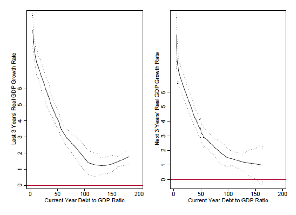
Moreover, a disproportionate number of the Japanese data points are extreme outliers – at both ends of the debt-to-GDP spectrum. A small number of extreme Japanese data points have an outsized influence for predictions of growth at both very high and at very low government debt-to-GDP ratios. Put simply, no other country in Reinhart’s and Rogoff’s 20 country dataset looks at all like Japan. To understand why, we will very briefly summarize relevant post-World War II Japanese economic history.
In 1942, Japan defaulted on bonds owned by Allied nations, because it was engaged in total war. As the war in the Pacific ground on, Japan’s government debt-to-GDP ratio shot upwards, until it reached about 200%. At that point, the allied bombing raids which destroyed much of urban and industrial Japan set off hyperinflation, which rapidly brought Japan’s government debt-to-GDP ratio down all the way to about 10%. As Reinhart and Rogoff themselves note in their paper, “The Forgotten History of Domestic Debt” (2008), “Domestic public debt was almost 80 percent of total domestic liabilities (including currency) in 1945 Japan, when inflation went over 500 percent.” At the same time, the destruction of much of Japan’s capital stock meant that after the war ended, Japan was poised to achieve high rates of growth in part simply from rebuilding what had been destroyed, as well as by adopting foreign technology and building up its export sector.
Figure 3: Japanese Government Debt-to-GDP ratio, 1885-2010
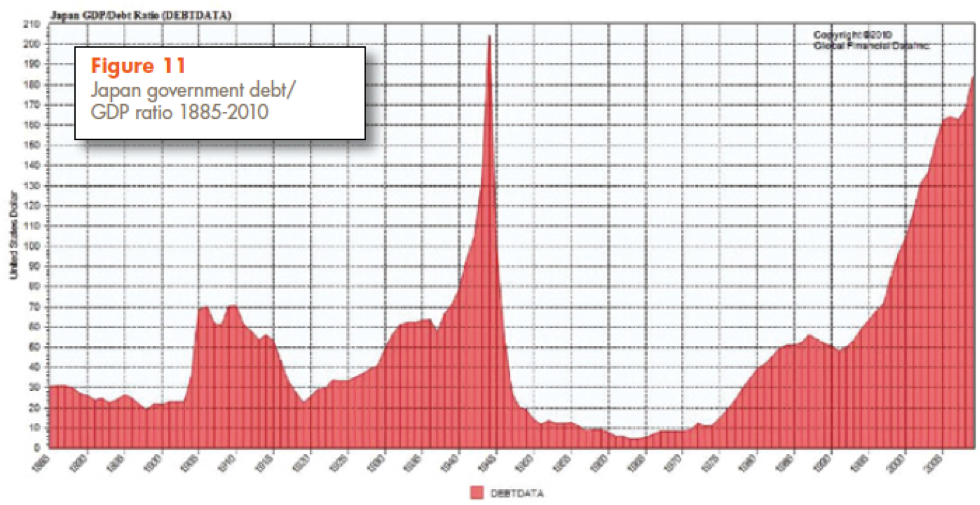
Hence the Japanese economy – and the government debt-to-GDP ratio – essentially re-started from scratch following Japan’s defeat in World War II. If Japan had been on the Allied side in World War Two, it most likely would have exited World War II with a very high government debt-to-GDP ratio, as did countries like the US and Australia. And then, as was the case in the US and Australia, the debt-to-GDP ratio would likely have fallen during the post-war boom. But because of its disastrous defeat, Japan entered the post-war era with an extremely low government debt-to-GDP ratio.
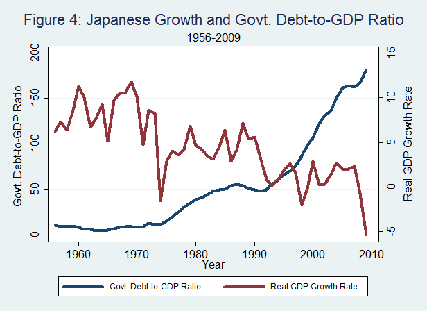
From 1956 (when Reinhart and Rogoff’s dataset commences) to 1971, as Japan rebuilt its economy, the average GDP growth rate was a very high 8.7% and the average government debt-to-GDP ratio was just 7.7%. From 1971 to 1990, the Japanese economy slowed down a bit but maintained strong positive growth. Then, from 1991 to 2000, following the collapse of Japan’s real estate bubble, Japan’s economy grew at just a 1.2% average rate, while the debt-to-GDP ratio averaged 72 (increasing throughout the period). And from 2001 to 2009, Japan grew at an average rate of .5%, while the debt-to-GDP ratio averaged 153 (again increasing throughout the period). Although the data does not go past 2009, Japan’s “lost” period is now approaching a quarter-century.
In the graph below, we can see that this history adds up to a very strong negative relationship between Japan’s GDP growth rate and its government debt-to-GDP ratio:
But Japan is perhaps the clearest of all examples of backwards-causation. In the case of Japan, the reason why the debt-to-GDP ratio has gone up so much in recent decades is that the Japanese economy has barely grown. And the reason why, from the end of World War II until 1970, the debt-to-GDP ratio was so low was that (as a legacy of the fact that it lost World War II), it started with a low government debt-to-GDP, and then it was able to grow very quickly by rebuilding what had been destroyed. As Paul Krugman (2013) has explained, (emphasis added):
“As soon as the paper was released, many economists pointed out that a negative correlation between debt and economic performance need not mean that high debt causes low growth. It could just as easily be the other way around, with poor economic performance leading to high debt. Indeed, that’s obviously the case for Japan, which went deep into debt only after its growth collapsed in the early 1990s.”
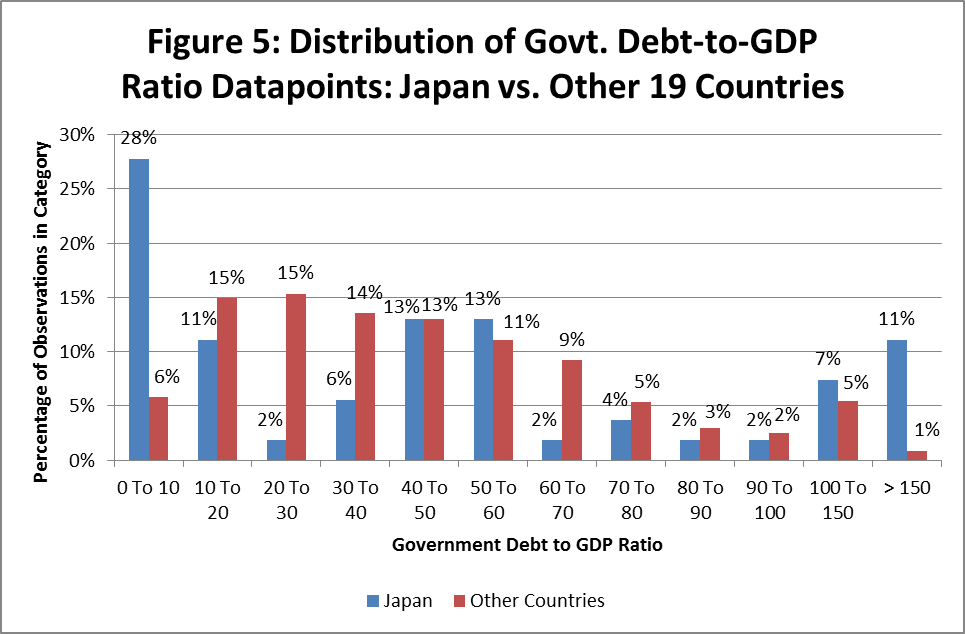
At least as importantly, the Japanese data are chock full of extreme outliers. This is not surprising given the economic history and the chart above, but we can see more clearly the sort of effect that Japanese data have on the overall picture by comparing the distribution of government debt-to-GDP ratio data points directly, between Japan and all the other 19 countries in the dataset:
Note that the Japanese outliers at high debt-to-GDP ratios appear less extreme in the chart above than they actually are because the high-end data are condensed into debt-to-GDP ratio buckets of 100 to 150 and > 150.
Data for the 19 non-Japan countries is strongly clustered in the range of a debt-to-GDP ratio from about 10% to 60%. But whereas the distribution of data for these 19 countries looks at least vaguely like a “bell curve,” the Japanese data have “fat tails.” Overall, 77% of non-Japanese lie within a debt-to-GDP ratio of 10% to 70%. But only 46% of the Japanese observations lie within that same 10% to 70% range.
28% of the Japanese data points are outliers on the low side, in the 0% to 10% debt-to-GDP ratio category. As is obvious from the rudimentary account of post-war Japanese economic history above, this data all comes from the early post-war era, when Japan was rebuilding out of the ashes of World War II and when Japan had very high and sustained growth rates. These observations from the period of Japan’s post-war “economic miracle” thus exhibit a strong tendency to tug estimated growth at low debt-to-GDP ratios sharply upwards.
Another 26% of the Japanese data points are on the high side, at debt-to-GDP ratios of greater than 70%. And at the far extreme end of the distribution, 11% of the Japanese data points are from debt-to-GDP ratios above 150%, while only 1% of the non-Japanese data points are from debt-to-GDP ratios above 150%. All the Japanese data points with high debt-to-GDP ratios stem from the lost quarter-century, and hence are associated with low growth rates. These data points thus exert a strong force pulling down any estimates of growth at high debt-to-GDP ratios.
LOWESS Regression Showing the Relationship Between Current Debt-to-GDP Ratio and Past/Future Growth
Using Dube’s stata .do file, we re-ran his analysis excluding Japan, thereby indirectly determining what effect Japanese data has upon the analysis. To emphasize, it is not valid to simply exclude Japanese data. Instead, the point is to indirectly see just how strong of an impact Japanese data have on the overall picture, and the point is that the strength of Japan’s effect leads one to anticipate that further analysis is likely to confirm the reverse causation hypothesis.
In Figure 6 below is a 19 country “backward/forward” LOWESS chart, which is exactly the same as a 20 country “backward/forward” LOWESS chart produced by Dube, except it does not include data from Japan. This chart shows the relationship between current year’s debt-to-GDP ratio and the last 3 years’ average GDP growth (on the left) and the relationship between current year’s debt-to-GDP ratio and the next 3 years’ average GDP growth (on the right).
Figure 6: Future and Past Growth Rates and Current Government Debt-to-GDP Ratio (Excluding Japan)
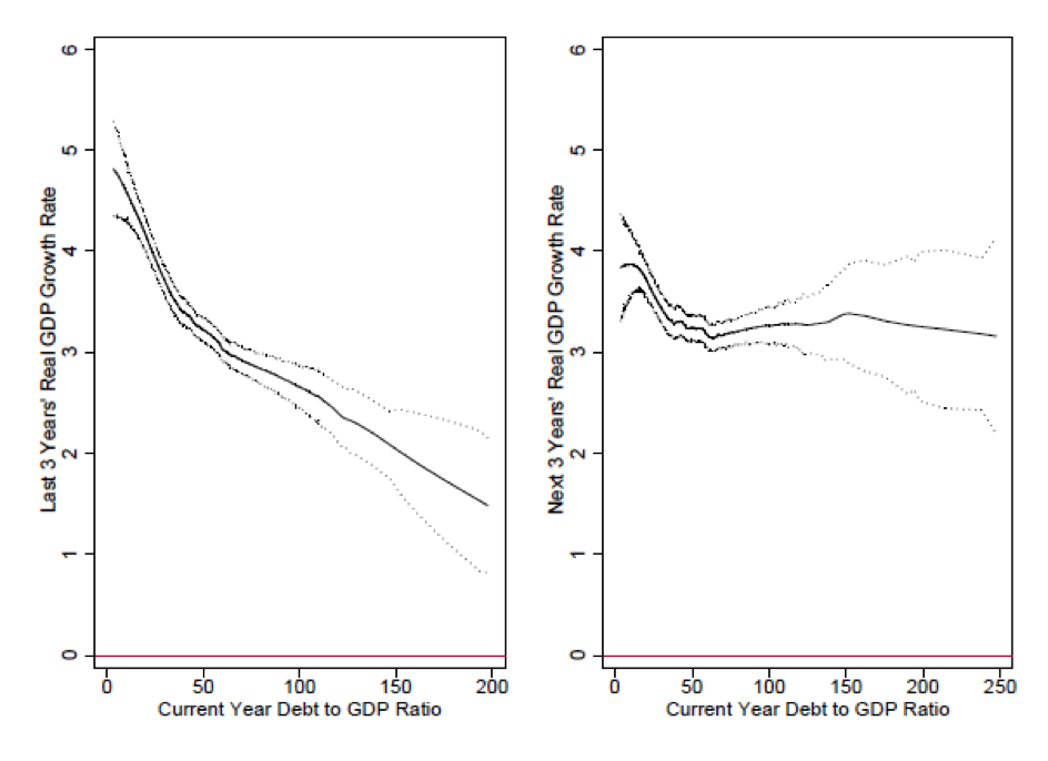
One can see from the left-side graph that a clear negative relationship between current year debt-to-GDP ratio and past growth is preserved, suggestive of reverse causality. But from the right-side graph, the relationship between current year debt-to-GDP ratio and future growth no longer looks at all negative, but rather is quite flat. This means that the (small) negative relationship between current year debt-to-GDP ratios and future growth which was preserved in Dube (2013) appears to be either mostly or entirely driven by Japan.
To facilitate a direct comparison between Dube’s original chart which includes all 20 countries and our chart which includes 19 countries (all except Japan), Figure 7 provides a side-by-side comparison.
Figure 7: Relationship Between Future Growth and Current Debt-to-GDP Ratio – Side-By-Side Comparison Including and Excluding Japan
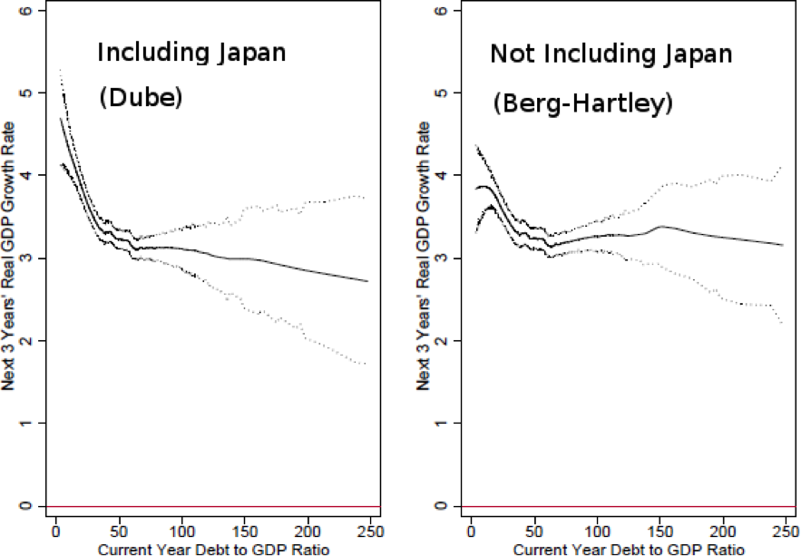
As we can see in Dube’s original chart (to the left), which includes Japan, there seems to be a fairly weak but nonetheless visible negative relationship between current year debt-to-GDP ratio and next 3 years’ GDP growth rate. This relationship is by far the strongest at low debt-to-GDP ratios, which does not make sense under the forward causation hypothesis.
But excluding Japan, one can see (in the chart to the right) that if there was previously a negative relationship, it all but vanishes. The chart excluding Japan is still very slightly downward sloping at very low debt-to-GDP ratios. From debt-to-GDP ratios of 50 until about 150, the line is essentially flat but slopes very slightly upwards. And from debt-to-GDP ratios of 150 to 250, the line is likewise essentially flat but slopes very slightly downwards. But at high (and low) debt-to-GDP ratios, 95% confidence bands widen substantially because there is less data available at the extremes. For all practical purposes, the chart excluding Japan is a flat horizontal line. This indicates that to the degree Dube (2013) provides evidence of a relationship between current year debt-to-GDP ratio and future growth, that evidence comes from – of all countries – Japan.
Impulse Response of GDP From Dube’s Distributed Lag Model
Next we use a distributed lag model and determine the impulse response of GDP growth if we do not include Japan (for a 10 point increase in the debt-to-GDP ratio). This is a more sophisticated way to look at the data than the LOWESS regressions above, because it gets a bit closer to the question of causation (though in reality, this looks at the relationship between variables through time, which is not necessarily the same thing as causation).
If we are correct in thinking that Japanese outliers are skewing the LOWESS regressions, then the distributed lag model may do a better job at picking up and correcting for the skew. But on the other hand, since Japan is an obvious case of reverse causality, if the backwards looking impulse response is substantially different when excluding Japan, then that would be bad news for the reverse causation explanation. But what we find is that the impulse response graphs look almost identical regardless of whether or not Japan is included. This is true both with and without fixed effects, as one can see from the side-by-side comparisons in Figures 8 and 9 below:
Figure 8: Impulse Response of GDP Growth from a 10-point increase in Government Debt-to-Income Ratio: Side-By-Side Comparison Including and Excluding Japan
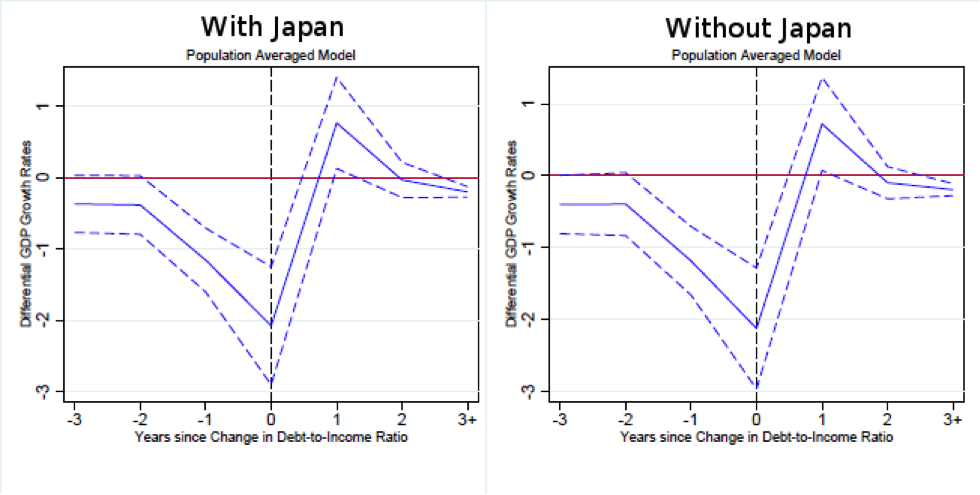
Figure 9: Impulse Response of GDP Growth from a 10-point increase in Government Debt-to-Income Ratio (With Fixed Effects): Side-By-Side Comparison Including and Excluding Japan
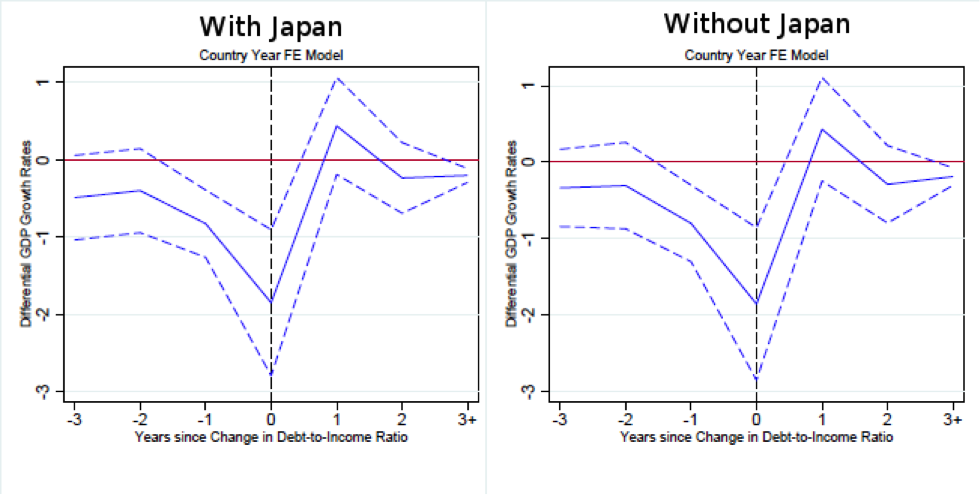
So, it appears that the impulse response results in Dube (2013) are not merely attributable to the influence of Japan (an obvious case of reverse causation). The evidence which seems to suggest reverse causation is apparently more deeply rooted across other countries, and not just in Japan. That evidence is clearly visible in the fact that in all of these impulse response graphs, the blue line is lower on the left (for years in the past) than on the right (for years in the future). This is also consistent with findings from Basu’s(2013) VAR models.
LOWESS Regression With Control For 1-Year Lagged GDP Growth
Finally, again following Dube (2013), we apply a LOWESS model excluding Japan. The result is Figure 10, which shows the relationship between current year debt-to-GDP ratio and current year GDP growth rate, both with no control (left) and with using 1-year lagged GDP growth as a control variable.
Figure 10: Current Growth Rate and Current Government Debt-to-GDP Ratio, Without and With Control for 1-year Lagged GDP Growth
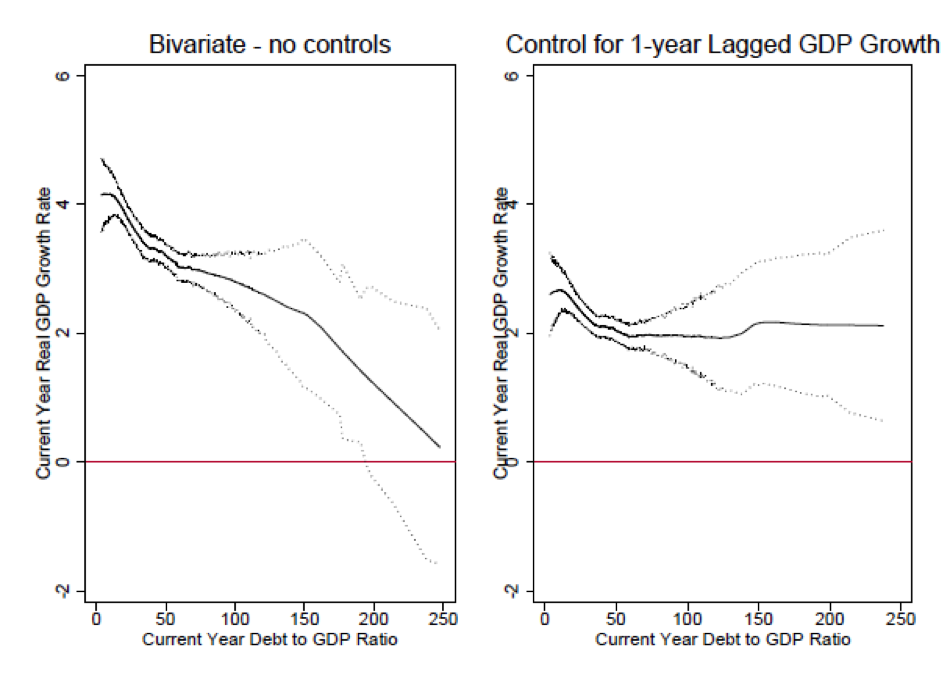
Unsurprisingly, we can see in the graph on the left that without any control, there is a negative overall correlation between the current year growth rate and the current year debt-to-GDP ratio. There is no dispute about that – the question is whether that relationship is the result of forward causation, or of backwards causation.
Once again, we will use a side by side comparison of Dube (2013)’s chart (including Japan) and our chart (excluding Japan) to make Japan’s impact on the overall analysis plain:
Figure 11: Current Growth Rate and Current Government Debt-to-GDP Ratio, Without and With Control for 1-year Lagged GDP Growth: Side-By-Side Comparison Including and Excluding Japan
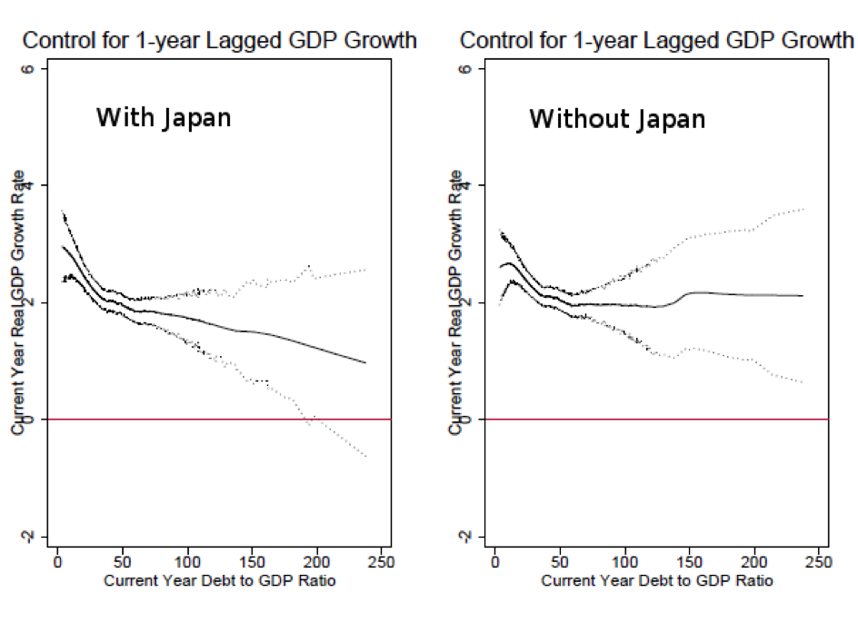
It is true that in Dube’s original chart (on the left) the negative relationship between current year real GDP growth rate and current year debt-to-GDP ratio is weak enough that it might not even exist (given the wide confidence bands). However, the chart may give the impression of a downward sloping relationship.
But when Japan is excluded (on the right), the regression line undeniably becomes quite flat. To be sure, the regression line on the right (without Japan) is not perfectly flat and horizontal. The line goes very slightly down at first until approximately a debt-to-GDP ratio of 30, then flattens out until about 150, then goes very slightly upwards, and then flattens out again. But for all practical purposes, this is about as flat a line an econometrician will ever obtain.
It appears, once again, that any small negative relationship between current year debt-to-GDP ratio and current year growth is a Japanese phenomenon – and given the results of VAR analysis on Japan in Basu (2013), that fact illuminates the issue of reverse causality vs. forward causality.
More analysis is still needed to fully confirm that the forward causation hypothesis is unfounded, and to further explore hints suggestive of reverse causation. VAR models ultimately only tell us whether one variable precedes another variable (which is not the same thing as causation) and can be vulnerable to omitted variables. Famously, Sims (1980) discovered that including the short term interest rate as a variable in his VAR model resulted in a complete reversal of his conclusions, from supporting “Monetarism” to supporting “Keynesianism.” So in addition to VAR models, simultaneous equations models and other methods may offer further evidence on the question of reverse causality.
Perhaps more importantly, as Nersisyan and Wray (2010) point out, the argument that high ratios of government debt-to-GDP cause low growth remains plagued by misconceptions, at least for nations which issue their own currency. Investigating differences between alternative monetary regimes, including the unit of account in which sovereign debts are denominated, provides an interesting avenue for further exploration.
We would like to thank Dr. Peter Eaton for his very valuable comments.
References:
Basu, Deepankar. (2013, Apr. 17) “The Time Series of High Debt and Growth in Italy, Japan, and the United States.”
http://www.nextnewdeal.net/rortybomb/guest-post-time-series-high-debt-and-growth-italy-japan-and-united-states
Dube, Arindrajit. (2013, Apr. 22) “Reinhart/Rogoff and Growth in a Time Before Debt.”
http://www.nextnewdeal.net/rortybomb/guest-post-reinhartrogoff-and-growth-time-debt.
Herndon, T., Ash, M., and Pollin, R. 2013 “Does High Public Debt Consistently Stifle Economic Growth? A Critique of Reinhart and Rogoff.” Political Economy Research Institute at University of Massachussetts Amherst,
http://www.peri.umass.edu/236/hash/31e2ff374b6377b2ddec04deaa6388b1/publication/566/.
Krugman, Paul. (2013, Apr. 19). “The excel depression: Commentary.” New York Times, pp. A.31.
http://www.nytimes.com/2013/04/19/opinion/krugman-the-excel-depression.html.
Nersisyan and Wray. (2010) “Does Excessive Sovereign Debt Really Hurt Growth? A Critique of This Time Is Different , by Reinhart and Rogoff.” Working Paper No. 603, Levy Economics Institute of Bard College,
http://www.levyinstitute.org/pubs/wp_603.pdf.
Reinhart, C. M. and Rogoff, K. S. (2010a). “Growth in a Time of Debt.” American Economic Review: Papers & Proceedings, 100.
http://www.aeaweb.org/articles.php?doi=10.1257/aer.100.2.573.
Reinhart, C. M. and Rogoff, K. S. (2010b). “Growth in a Time of Debt.” Working Paper 15639, National Bureau of Economic Research,
http://www.nber.org/papers/w15639.
Reinhart, C. M. And Rogoff, K. S. (2013, Apr. 25). “Reinhart and Rogoff: Responding to Our Critics.” New York Times.
http://www.nytimes.com/2013/04/26/opinion/reinhart-and-rogoff-responding-to-our-critics.html?pagewanted=all.
Reinhart, C. M. and Rogoff, K. S. (2008). “The Forgotten History of Domestic Debt.” Working Paper 13946, National Bureau of Economic Research,
www.nber.org/papers/w13946.
Reinhart, C. M. and Rogoff, K. S. (2009) This time is different: Eight centuries of financial folly, Princeton University Press.
Sims, C. A. (1980). “Comparison of interwar and postwar business cycles: Monetarism reconsidered.” The American Economic Review, 70(2), 250-257.



Pingback: Austerity leads to...austerity! - Forbes
Pingback: Make ‘em Prove the Causality before They Cause Any More Suffering: Part One | New Economic Perspectives
Pingback: Make ‘em Prove the Causality before They Cause Any More Suffering: Part Two, the Fall and After | New Economic Perspectives
Pingback: Make ‘em Prove the Causality before They Cause Any More Suffering: Part Three, Reinhart - Rogoff Retrospective | New Economic Perspectives
Pingback: | New Economic Perspectives