Category Archives: Eric Tymoigne

MMT 101: Response to the Critics Part 2

The Simplest Case: The Circuit with a Consolidated Government

By  Eric Tymoigne and L. Randall Wray

[Part I] [Part II] [Part III] [Part IV] [Part V] [Part VI]

MMT is frequently criticized for consolidating the treasury and the central bank. (Palley 2012; JKH 2012a, 2012b; Lavoie 2013; Fiebiger 2012a, 2012b; Rochon and Vernango 2003; Gnos and Rochon 2002). They note that this hypothesis does not describe the current institutional framework of developed countries, and claim it pushes MMT into unnecessary strong logical claims. In this post, we will address these issues by tackling problems surrounding the nature of money and the role of taxes, and by beginning to deal with the consolidation argument.

The theory of the circuit discussed in Part 1 is a good starting point. Like all theories, it simplifies the existing economic system in order to draw causalities from logical reasoning. From the circuit theory, one can better understand Keynes’s point that spending is what makes saving possible (Keynes 1939), and the importance of distinguishing financing (initial finance) from funding (final finance). Parguez (2002) and Bougrine and Seccareccia (2002) have shown how the circuit theory can be extended to include the state, and reached similar conclusions to MMT.

Continue reading

MMT 101: A Reply to Critics Part 1

By  Eric Tymoigne and L. Randall Wray

[Part I] [Part II] [Part III] [Part IV] [Part V] [Part VI]

This is Part 1 of a six part series in which we deal with critics of MMT. As readers of this blog know, our critics continually raise the same old tired critiques of MMT. They scapegoat MMT by attributing to us claims we’ve never made. They take our words out of context to build up a strawman that they attempt to destroy. No matter how many times we respond to a particular critique, another critic tries to use it again. Warren Mosler used to use the analogy of the “Bop a Gopher” game at the arcades: you bop one and another pops up.

While we know that it’s a Sisyphean task to disabuse the critics of their cherished and wrong-headed arguments, we thought it would be useful for those who come to MMT with less prejudice to have at hand responses to five categories of critiques. Today we will provide an introduction to the series. Each of the next five posts will deal with one of the critiques. We’ll also append a list of the references used for this entire series.

Continue reading

Public Debt, Debt Ceiling and Monetary Sovereignty: Some Accounting Realities

By Eric Tymoigne

The public debt is the outstanding U.S. Treasury securities (USTS). It includes both marketable (T-bills, T-notes, T-bonds, TIPSs, and a few others) and non-marketable securities (United States notes, Gold certificates, U.S. savings bonds, Treasury demand deposits issued to States and Local Gov., all sorts of government account series securities held by Deposit Funds). What are the means to reduce the public debt? Continue reading

Unjustified Fears over Sovereign Debt

By Nora Apter

Another great video by a student in Eric Tymgoine’s modern money course.

Sovereign Currency Issuers Are Always Solvent

By Joseph Hykan

Another great video developed for Eric Tymgoine’s modern money course.

After Great Recession: A Bleaker Employment Recovery than after the Great Depression

By Eric Tymoigne

The last employment numbers provide yet another disappointing bit of news for millions of households all around the country. No net employment gain. However, I am afraid that this is only the very tip of the iceberg because a long-term view shows a much bleaker picture.

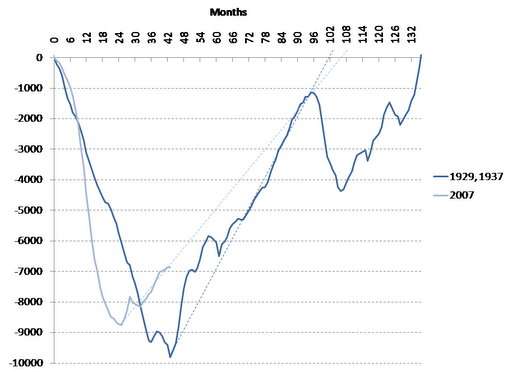
Figure 1 shows how long it took for the employment level to return to its peak level after a recession, and how much job loss occurred relative to that peak. The employment numbers exclude people that were employed in the WPA, NYA and CCC, and focuses on individuals employed in nonfarm activities.

During the Great Depression, the employment level declined for 4 years and almost 10 million jobs were lost compared to the peak employment level that prevailed in August 1929. It took 136 months (over 11 years) to return to this level of employment, but, without the avoidable 1937 recession, the full recovery would have occurred after 102 months (8.5 years) if one takes the trend of recovery that prevailed from 1933.

The Great Recession led to a loss of almost 9 million jobs compared to the peak employment level of January 2008. The loss of jobs occurred at a faster rate than the Great Depression but employment recovered sooner and started to rise after 2 years. However, once the employment recovery started, it occurred at a slower rate than during the Great Depression. If the recovery continues at the same pace, AND assuming that no recession occurs during the recovery phase, it will take about 9 years to return to the employment level of January 2008. Thus, given everything else, it will take longer for employment to fully recover than during the years prior to the 1937 recessions.

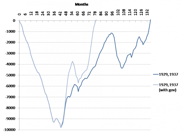
The picture is even bleaker today if one included New Deal employment programs. Figure 2 shows that those programs allowed employment to recover fully after 80 month (less than 7 years) and only three years after the New Deal Programs were implemented. The timid Bush and Obama stimulus have barely made a dent in the employment problem over the past two years.

This, once again, suggest a powerful employment policy to help the economy. Instead of concentrating its efforts on tax rebates and bailing out banks, and waiting for them to lend to businesses, the federal government should directly hire people and involve them in activity that benefited the entire country. We do not need a temporary stimulus; we need a permanent institutionalized and decentralized government program that hires anybody willing to work and unable to find a job in the private sector. By sustaining income and the productivity of workers, a government employment program would tremendously helps to sustain the employability of workers and would improve the confidence of private business, which would in turn improve private employment.

Figure 1. Difference between peak employment level and current employment level. Nonfarm payroll employment, seasonally adjusted, millions of people.


Sources: BLS (Current Employment Survey), Federal Reserve Bulletin (June and September 1941).
Note: People employed in the WPA, NYA and CCC are not included.

Figure 2. Same as Figure 1 with New Deal Federal Employment Programs.

Sources: Federal Reserve Bulletin, Social Security Bulletin.

Where is the “Recovery”? Where Did the “Stimulus” Go?


The new BEA figures about economic activity continue to point to a replay of a Japanese-style lost decade or, even worse, a 1937 scenario. The current expansion has been the weakest on record since World War Two and the trend since the early 1980s does not provide much comfort. Figure 1 shows that each economic expansion since the 1980s has been weaker and weaker and the rate of decline has accelerated.

The current debate in Washington does not provide any comfort for the short run or the long run with both political parties willing to jeopardize whatever economic growth we have left over a fictitious ceiling that serves no economic purpose. All this suffering is supposed to help in the long run because of the good that will come from “reforming” (read “dismantling”) pillars of economic progress like Social Security.

The 2009 Obama “stimulus” is long gone and all levels of government negatively contributing to economic growth. Since the third quarter of 2009, the contribution of the government to economic growth has been nil on average. 

Two Theories of Prices

Last May, John T. Harvey wrote a wonderful post about the quantity theory of money (QTM). This post picks up where John stopped, presenting a different theory of the price level and inflation. It’s a bit technical (so bare with me), but many readers have asked us to elaborate on price theory.
First, a quick recap. The QTM starts with the identity MV ≡ PQ, where M = the money supply, V = the velocity of money, P = the price level, and Q = the quantity of output (Fisher’s version is broader and includes all transactions: T). The identity is a tautology, it just says that the amount of transactions on goods and services (PQ) is equal the to the amount of financial transactions needed to complete those transactions. To get a theory of price (the QTM), one must make some assumptions about each variable. The QTM assumes that:
·         M is constant (or grows at a constant rate) and is controlled by the central bank through a money multiplier
·         V is constant
·         Q is constant at its full employment level (Qfe) or grows at its natural rate (gn)
Given this set of assumptions, we get (note the equality sign to signal causality):
P = MV/Qfe
Or, in terms of the growth rate (V is constant so its growth rate is zero):
gp = gm – gn
This is the QTM, which holds that price changes (inflation and deflation) have monetary origins, i.e. if the money supply grows faster than the natural rate of economic growth, there is some inflation.  For example, if gm = 2% and gn = 1% then gp = 1%.  If the central bank increases the money supply, then inflation rises.

John’s post explains the problems with this theory. M is endogenous, V is not constant, and the economy is rarely at full employment. If you want to know more, you should read John’s post.

Let’s move to an alternative theory of the price level and inflation by starting with another identity based on macroeconomic accounting:
PQ ≡ W + U
This is the income approach to GDP used by the Bureau of Economic Analysis. It says that nominal GDP (PQ) is the sum of all incomes. For simplicity, there are only two incomes: wage bill (W) and gross profit (U). Both are measured before tax.
Let’s divide by Q on each side:
P ≡ W/Q + U/Q
We can go a bit further by noting that W is equal to the product of the average nominal wage rate and the number of hours of labor W = wL (for example, if the wage rate is $5 per hour, and L is equal to 10 hours, then W is equal to $50). Thus:
P ≡ wL/Q + U/Q
Q/L is the quantity of output per labor hour, also called the average productivity of labor (APl) therefore:
P ≡ w/APl + U/Q
w/APl is called the unit cost of labor and data can be found at the BLS. The term U/Q will be interpreted a bit later.
Ok let’s stop a bit here. For the moment all we have done is rearranged terms, we have not proposed a theory (i.e. a causal explanation that provides behavioral assumptions about the variables.)  Here they are:
·         The economy is not at full employment and Q (and economic growth) changes in function of expected aggregate demand (this is Keynes’s theory of effective demand).
·         w is set in a bargaining process that depends on the relative power of workers (the conflict claim theory of distribution underlies this hypothesis)
·         U, the nominal level of aggregate profit, depends on aggregate demand (Kalecki’s theory of profit underlies this hypothesis)
·         APl moves in function of the needs of the economy and the state of the economy.
Thus we have:
P = w/APl + U/Q
Thus the price level changes with changes in the unit cost of labor and the term U/Q. What is this last term? To understand it let’s express the previous equation in terms of growth rate. This is approximately:
gp = (gw – gAPl)sW + (gU – gQ)sU
With sW and sU the shares of wages and profit in national income (sW + sU = 1).
Thus, inflation will move in relation to the growth rate of the unit labor cost of labor, which itself depends on how fast nominal wages grow on average relative to the growth rate of the average productivity of labor. As shown in the following figure, in the United States, a major source of inflation in the late 1960s and 1970s was the rapid growth of the unit cost of labor, with the rate of change between 5 and 10 percent.

Major Sector Productivity and Costs Index (BLS)

Series Id:  PRS85006112
Duration:   % change quarter ago, at annual rate
Measure:    Unit Labor Costs
Sector:     Nonfarm Business
Inflation will also move in relation to the difference between the growth rate of U and the growth rate of the economy (gQ). U follows Kalecki’s equation of profit, which broadly states that that the level of profit in the economy is a function of aggregate demand. Thus the term, (gU – gQ) represents the pressures of aggregate demand on the economy. If gU goes up and gQ is unchanged, then gP rises given everything else. However, to assume that gQ is constant is not acceptable unless the economy is at full employment, so a positive shock on aggregate demand will usually lead to a positive increase in gQ.
Thus, overall, there are two sources of inflation in this approach, a cost-push source (here summarized by the unit labor cost) and a demand-pull source (here summarized by the aggregate demand gap). Note that the money supply is absent from this equation. Money does not directly affect prices. Assuming that a drop of money from the sky leads to inflation, first, does not understand how the money supply is created (it is at least partly created to produce goods and services), second, assumes that people will automatically spend rather than hoard the addition funds obtained (people do hoard for all sorts of reasons and do derive “utility” from hoarding money), third, assumes that the economic output cannot respond to additional demand. If more people suddenly go to the store, producers usually produce more rather than raise prices. Output is not a fixed pie that involves allocation to one group at the expense of another group. The size of the pie increases and decreases with the number of people demanding pie.
A version of this theory has been used in many different models that have endogenous money, liquidity preference, demand-led theory of output and other non-mainstream characteristics. Godley’s and Lavoie’s Monetary Economics as well as Lavoie’s Foundation of Post Keynesian Economics are good books to get more modeling. Of course, modern mainstream monetary economics is rejected in those books; income effect dominates over substitution effect, production is emphasized over allocation, monetary profit affects economic decisions, etc. Be prepared for a change of perspective in which scarcity is not the starting point of economics.

$50 Billion in Infrastructure Spending: A drop in the Bucket

The White House released the following statement regarding its new recovery plan: “The President today laid out a bold vision for renewing and expanding our transportation infrastructure – in a plan that combines a long-term vision for the future with new investments. A significant portion of the new investments would be front-loaded in the first year.”
This front load is worth $50 billion…a lot of money…but an insignificant amount compared to the size of what is needed. It is not a bold vision it is a very timid vision. Don’t believe me? Ask the American Society of Civil Engineers. In its 2009 Infrastructure Report Card, it gave a D average to US infrastructures and recommended $2.2 trillion of dollars of spending over the next 5 years. And that is just to bring current infrastructures back to good condition; trillions more are needed to respond to growing needs.

Money is not a problem for the federal government, all this could be started tomorrow like we have done to finance wars, bail outs the financial sector and other wasteful items. We did it before, when the country had a truly bold vision and was much less wealthy, and we could do it again. Besides current infrastructures, we need to start to use our underused resources (especially labor) to address the future needs of our aging population and our environmental problems: education, infrastructure, social networks, technology, energy, food production, and many others sectors need help.

The CBO’s Misplaced Fear of a Looming Fiscal Crisis

By Eric Tymoigne

The Congressional Budget Office (CBO) has just released an 8-page brief titled “Federal Debt and the Risk of a Fiscal Crisis.” In it you will find all the traditional arguments regarding government deficits and debt: “unsustainability,” “crowding out”, bond rates rising to “unaffordable” levels because of fears that the Treasury would default or “monetize the debt,” the need to raise taxes to pay for interest servicing and government spending, the need “to restore investor’s confidence” by cutting government spending and raising taxes. This gives us an opportunity to go over those issues one more time.

  1. “growing budget deficits will cause debt to rise to unsupportable levels”

A government with a sovereign currency (i.e. one that creates its own currency by fiat, only issues securities denominated in its own currency and does not promise to convert its currency into a foreign currency under any condition) does not face any liquidity or solvency constraints. All spending and debt servicing is done by crediting the accounts of the bond holders (be they foreign or domestic) and a monetarily-sovereign government can do that at will by simply pushing a computer button to mark up the size of the bond holder’s account (see Bernanke attesting to this here).

In the US, financial market participants (forget about the hopelessly misguided international “credit ratings”) recognize this implicitly by not rating Treasuries and related government-entities bonds like Fannie and Freddie. They know that the US government will always pay because it faces no operational constraint when it comes to making payments denominated in a sovereign currency. It can, quite literally, afford to buy anything for sale in its own unit of account.


This, of course, as many of us have already stated, does not mean that the government should spend without restraint. It only means that it is incorrect to state that government will “run of out money” or “burden our grandchildren” with debt (which, after all, allows us to earn interest on a very safe security), arguments that are commonly used by those who wish to reduce government services. These arguments are not wholly without merit. That is, there may well be things that the government is currently doing that the private economy could or should be doing. But that is not the case being made by the CBO, the pundits or the politicians. They are focused on questions of “affordability” and “sustainability,” which have no place in the debate over the proper size and role for government (a debate we would prefer to have). So let us get to that debate by recognizing that there is no operational constraint – ever – for a monetarily sovereign government. Any financial commitments, be they for Social Security, Medicare, the war effort, etc., that come due today and into the infinite future can be made on time and in full. Of course, this means that there is no need for a lock box, a trust fund or any of other accounting gimmick, to help the government make payments in the future. We can simply recognize that every government payment is made through the general budget. Once this is understood, issues like Social Security, Medicare and other important problems can be analyzed properly: it is not a financial problem; it is a productivity/growth problem. Such an understanding would lead to very different policies than the one currently proposed by the CBO (see Randy’s post here).

  1. “A growing portion of people’s savings would go to purchase government debt rather than toward investments in productive capital goods such as factories and computers.”

First, this sentence seems to imply that government activities are unproductive (given that, following their logic, Treasury issuances “finance” government spending), which is simply wrong, just look around you in the street and your eyes will cross dozens of essential government services.

Second, the internal logic gets confusing for two reasons. One, if people are so afraid of a growing fiscal crisis, why would they buy more treasuries with their precious savings? Why not use their savings to buy bonds to fund “productive capital goods”? Using the CBO’s own logic, higher rates on government bonds would not help given that a “fiscal crisis” is expected and given that participants are supposed to allocate funds efficiently toward the most productive economic activity (and so not the government according to them). Second, we are told that “it is also possible that investors would lose confidence abruptly and interest rates on government debt would rise sharply.” I will get back to what the government can do in that case, but you cannot get it both ways; either financial market participants buy more government securities or they don’t.

Third, this argument drives home the crowding-out effect. I am not going to go back to the old debates between Keynes and others on this, but the bottom line is that promoting thriftiness (increasing the propensity to save out of monetary income) depresses economic activity (because monetary profits and incomes go down) and so decreases willingness to invest (i.e. to increase production capacities). In addition, by spending, the government releases funds in the private sector that can be used to fund private economic activity; there is a crowding-in, not a crowding-out. This is not theory, this is what happens in practice, higher government spending injects reserves and cash in the system, which immediately places downward pressure on short-term rates unless the Fed compensates for it by selling securities and draining reserves (which is what the Fed does on a daily basis).

  1. “if the payment of interest on the extra debt was financed by imposing higher marginal tax rates, those rates would discourage work and saving and further reduce output.”

No, as noted many times here, all spending and servicing is done by crediting creditor’s account not by taxing (or issuing bonds). Taxes are not a funding source for monetarily-sovereign governments, they serve to reduce the purchasing power of the private sector so that more real resources can be allocated to the government without leading to inflation (again all this does not mean that the government should raise taxes and takeover the entire economy; it is just a plain statement of the effects of taxation). All interest payments on domestically-denominated government securities (we are talking about a monetarily-sovereign government) can be paid, and have been met, at all times, whatever the amount, whatever their size in the government budget.

  1. “a growing level of federal debt would also increase the probability of a sudden fiscal crisis, during which investors would lose confidence in the government’s ability to manage its budget, and the government would thereby lose its ability to borrow at affordable rates.”

If the US Treasury cannot issue bonds at the rate it likes there is a very simple solution: do not issue them. This does not alter in any way its spending capacity given that the US federal government is a monetarily-sovereign government so bond issuances are not a source of funds for the government. Think of the Federal Reserve: does it need to borrow its own Federal Reserve notes to be able to spend? No, all spending is done by issuing more notes (or, more accurately, crediting more accounts) and if the Fed ever decided borrow its own notes by issuing Fed bonds to holders of Federal Reserve notes (a pretty weird idea), a failure of the auction would not alter its spending power. The Treasury uses the Fed as an accountant (or fiscal agent) for its own economic operations; the “independence” of the Fed in making monetary policy does not alter this fact.

  1. “It is possible that interest rates would rise gradually as investors’ confidence declined, giving legislators advance warning of the worsening situation and sufficient time to make policy choices that could avert a crisis.”

It is always possible that anything can happen, but what is the record? The record is that there is no relationship between the fiscal position of the US government and T-bond rates. Massive deficits in WWII went pari passu with record low interest rates on the whole Treasury yield curve. With the help of the central bank, the government made a point of keeping long-term rates on treasuries at about 2% for the entire war and beyond, despite massive deficits. There is a repetition of this story playing out right now, and Japan has been doing the same for more than a decade. Despite its mounting government debt, the yield on 10-year government bonds is not more than 2% as of July 2010. In the end, market rates tend to follow whatever the central bank does in terms of short-term rates, not what the fiscal position of the government is.

As we already stated on this blog before, a simple observation of how government finance operates shows that government spending injects reserves into the banking system (pressing down short-term interest rate), while the payment of taxes reduces/destroys reserves (pushing short-term rates up). The Fed has institutions that allow it to coordinate on a daily basis with the Treasury (they call each other every day) to make sure that all these government operations do not push the interest rate outside the Fed’s target range.

  1. “If the United States encountered a fiscal crisis, the abrupt rise in interest rates would reflect investors’ fears that the government would renege on the terms of its existing debt or that it would increase the supply of money to finance its activities or pay creditors and thereby boost inflation.”

That’s a repeat of the first question but with a bit of elaboration. The US government cannot default on its securities for financial reasons, it is perfectly solvent and liquid. (Sovereign governments can, as we have conceded on this blog, refuse to pay – e.g. Japan after the war – but that is because it was unwilling to repay, not because it was unable to pay.) Thus, despite Reinhart and Rogoff’s warnings, the credit history of the US government (and any monetarily-sovereign government) remains perfect. No government with a non-convertible, sovereign currency has ever bounced a check trying to make payment in its own unit of account.

The US government always pays by crediting the account of someone (i.e. “monetary creation”). If the creditor is a bank, this leads to higher reserves, if it is a non-bank institution it leads also to an increase in the money supply. It has been like this from day one of Treasury activities. It is not a choice the government can make (between increasing the money supply, taxing or issuing bonds); any spending must lead to a monetary creation; there is no alternative. Again taxes and bonds are not funding sources for the US federal government; however they have important functions. Taxes help to keep inflation in check (in addition to maintaining demand for the government’s monetary instruments). Bond sales allow the government to deficit spend without creating excessive volatility in the federal funds market. If financial market participants want more bonds, the Treasury issues more to keep bond rates high enough for its tastes; if financial market participants do not want more treasury bonds, the government does not issue to avoid raising rates. The US Treasury (and any monetarily sovereign government as long as they understand it) has total control over the rate it pays on its debts; whether the government understands this or not is another question. A monetarily sovereign government does not have to pay “market rates” in order to convince markets to hold its bonds. Indeed, it does not even have to issue securities if it does not want to. In the US, it is usually the financial institutions that beg the Treasury to issue more securities.

The recent episode of the “Supplementary Financing Program” is a very good illustration of that point. Financial market participants were crying for more Treasuries and the Fed could not keep pace. As a consequence the Treasury agreed to issue more Treasuries than expected to meet the demand and help the Fed drain reserves and thereby hit their interest rate target. According to the Federal Reserve Bank of New York (DOMESTIC OPEN MARKET OPERATIONS DURING 2008, page 28): “To help manage the balance sheet impact of the Federal Reserve’s liquidity initiatives, the Treasury announced the establishment of a temporary Supplementary Financing Program (SFP) on September 17. The program consists of a series of Treasury bills issued by Treasury, the proceeds of which are deposited in an account at the Federal Reserve, draining reserve balances from the banking sector.”

Now look how this was deformed by the Treasury (quite a few journalists and bloggers followed): “The Treasury Department announced today the initiation of a temporary Supplementary Financing Program at the request of the Federal Reserve. The program will consist of a series of Treasury bills, apart from Treasury’s current borrowing program, which will provide cash for use in the Federal Reserve initiatives.” No, Mr. Treasury, this was not done for funding purpose; it was done to drain reserves from the banking system. The Fed does not need any cash from the Treasury. The Fed is the monopoly supplier of cash.

A final point regarding inflation. Inflation is a potential issue, as we have always maintained. But, there is no automatic causation from the money supply to inflation (a point Paul Krugman appears to have forgotten). Inflationary pressures depend on the state of the economy (supply and demand-side factors). Most importantly, perhaps, it depends on people’s desire to hoard vs. spend cash. Even the massive deficits during WWII, when resources were fully employed, did not lead to a spiraling out of control of inflation. Finally, it is quite possible that causation actually runs the other way around – i.e. from inflation to the money supply – given the endogeneity of the money supply, but that’s a story for another day…