
By Eric Tymoigne
In Post 20, a lot is said about the role that the rate of return on financial instruments—the interest rate—plays on the pricing on securities, but little was said about what determines that rate of return. Two competing theoretical frameworks explain what influences the interest rate, one of them emphasizes the role of real factors and the other emphasizes monetary factors.
Real Theory of Interest Rate: Natural Interest Rate and Expected Inflation
Gross Substitution and Indifference Condition: Determinant of the Nominal Interest Rate
The real exchange framework (Post 12) emphasizes the role played by real variables in the decision-making process of any rational economic unit. People are not fooled by mere improvement in monetary income because they only care about improvement in purchasing power given that only consumption provides utility. Monetary instruments have no other purpose than to smooth market transactions, and preoccupation about the liquidity of balance sheets and monetary outcomes are irrelevant. Capitalism is equivalent to a barter economy that uses monetary instruments.
In the early 1900s, Irving Fisher provided a theory of the interest rate that is consistent with that framework. The theory starts with each economic unit maximizing its intertemporal utility by modifying its intertemporal real income to fit its preference in terms of intertemporal consumption. An economic unit does so by trading assets that earn a return while they are held. An economic unit buy assets that provides the highest rate of return and sell others. This arbitrage leads to an equalization of rates of return, at which point an economic unit is indifferent about holding any asset and so stop trading them.
A central hypothesis is that all assets are perfect substitutes so economic units are merely concerned with acquiring assets that provide the highest rate of return. The liquidity of assets is of no concern because there is no uncertainty. There exists a market for all potential future contingencies and so an economic unit can optimize its portfolio position to account for them. As such, assets like household appliances, houses, furniture, clothes and other goods and services are as reliable means to store value as financial instruments.
This microeconomic logic is generalized to the macroeconomic level. At that level, there are only two assets, a monetary asset and a commodity called real aggregate income (think of “potato”). The monetary asset provides a rate of return when it is lent. Real aggregate income provides a rate of return when it is invested, that is, used to grow productive capacities (plant the potatoes). The rate of return on aggregate income comes in the form of additional real aggregate income (more potatoes). In order to be able to compare the rate of return on both assets, one must use a common unit by calculating the nominal rate of return on real aggregate income. Once the two monetary rates of return are known, economic units perform an arbitrage between these two assets. The arbitrage continues until economic units are indifferent between monetary and non-monetary assets, which occurs when the nominal rates of return on both assets are equal:
it = rt* + Et(gP)
The rate of return on monetary assets is the nominal interest rate i. r* is the real rate of return on aggregate income, also called equilibrium real interest rate or the natural interest rate. Et(gP) is the current expectation about future inflation (gP is the growth rate of output price). rt* + Et(gP) is the expected monetary rate of return on non-monetary assets. One may note that the nominal rate of return on non-monetary assets does not include capital gains but merely reward in terms of physical income. This is consistent with the framework of the efficient market hypothesis and its focus on fundamental value (see Post 20).
If i is lower than rt* + Et(gP), it means that the cost of credit is lower than the nominal return on physical assets. In that case, deficit-spending economic units have an incentive to invest by borrowing monetary assets from savers (banks are merely intermediaries between savers and investors, see Post 10). The increase in spending leads to inflation, which pushes up the interest rate until it is equal to the expected monetary rate of return on real aggregate income. If i > rt* + Et(gP), borrowing falls, inflation falls, and so i falls until both rate of return are equal (Figure 21.1). Thus, in this theoretical framework, i adjusts to rt* + Et(gP) ; it is a real theory of interest rate. The following studies how each component of the monetary rate of return on non-monetary assets are determined.

Figure 21.1. Adjustment mechanism in the real exchange economy framework
Inflation Expectations
In terms of expected inflation, the theory of inflation associated with the real exchange economy framework is the quantity theory of money (Post 11):
gP = gM – gQfe
If the central bank loosens its policy—either through a higher reserves growth rate (see money multiplier theory in Post 10) or by lowering its interest rate—the growth rate of the money supply rises (gM goes up) and so inflation rises (gP goes up) because economic growth stays at its natural growth rate (gQfe). In short, too much money chasing too few goods causes inflation. As such, expected inflation depends on expected future monetary conditions and, if the central bank injects large amounts of excess reserves (Post 3), one can expect higher inflation and so higher interest rates:
E(gP) = E(gM) – gQfe
The natural rate of interest is the interest rate that keeps prices stable, that is the interest rate that leads to no inflation or deflation (gP = 0%). The natural rate of interest is set in the loanable funds market (Figure 21.2). According to the real exchange economy framework, the loanable funds market approximates financial markets. As explained in Post 12 and Post 20, in the real exchange economy framework, one can study capitalist economies as if they are barter economies, and financial markets are just a means to perform intertemporal barter in order to adjust intertemporal consumption according to someone’s preferences. Financial markets are just a means for economic units with a surplus of commodities (the savers) to lend them to economic units with a deficit of commodities (the investors). While all transactions are done in monetary forms, what is transferred is purchasing power and so ultimately goods and services. Savers gives up present consumption so that some goods and services can be allocated to increase the future production of goods and services (investment). Savers are rewarded for their patience with more consumption in the future and so saving is merely a signal of future consumption, which encourages firms to invest today to meet that future consumption. The role of financial markets is to find the equilibrium interest rate that ensures that saving equals investment, that is, that ensures that output grows enough to satisfy desired future consumption. To see this more clearly, the following studies each curve in more detail.
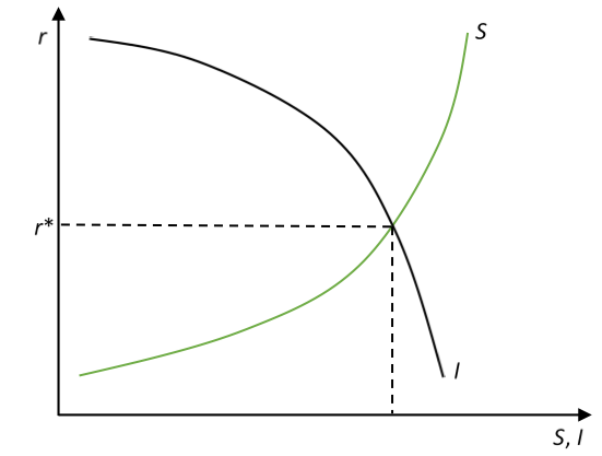
Figure 21.2. The loanable funds market
On the supply side are savers. Economic units receive an income and they have to decide if they should consume now or later. In order to decide about the mix of present and future consumption, economic units do not make a random decision. Their aim is to find the optimal mix, that is, the mix that maximizes their utility (happiness) over time. Economic units do so by comparing the reward they can get from saving one more dollar, to the pain induced by saving that additional dollar (delaying consumption is painful). They do this calculation for each dollar. The reward for saving one more dollar is the real interest rate r, some additional consumption in the future that is worth a certain amount of utils. The pain of saving one more dollar is the marginal disutility of waiting, which depends on the patience of each economic unit: individuals who are spendthrift feel a greater pain and have a pain that rises faster than individuals who are frugal. The supply of saving is upward slopping because the pain increases as more saving is done so the reward for saving more must be increased. The supply of curve is also convex, which reflects the acceleration in the pain felt.
On the demand side, there are investors who, to simplify, are considered to be businesses. Remember that investment in macroeconomics means building productive capacities (buying machines, increasing human capital by getting an education). Investing is expensive so economic units who want to do so need to borrow funds from savers. These borrowed funds allowed investors to buy the commodities that savers agree to let go at the present time. Once again, there is a calculation to perform in order to find the optimal level of investment, which is the level that maximize the real profit of firms. Businesses do so by comparing the benefit of investing one more dollar to the cost of investing that additional dollar. The reward is more output and this additional output is called the marginal product of capital, which is the output produced by one additional machine. The cost of investing one more dollar is the real interest rate: investors must give away some of the additional output produced in order to pay the interest income due to savers. Debt payments are measured in real terms and potentially performed in real terms (Post 12). The demand curve is downward slopping because the marginal product of capital falls as investment increases so the interest rate must decrease to make an additional investment profitable. The demand curve is also concave to reflect the fact that the marginal product falls more rapidly as investment increases.
From this presentation, one can conclude that two main factors influence the natural interest rate, time preference (patience of individuals) and technology (marginal product of capital). Monetary conditions have no influence on the natural rate. If individuals become less patient, they save less for each level of interest, that is, one must reward individuals more to save the same amount (Figure 21.3). The natural rate of interest rate increases with lower patience (higher preference for present consumption). If the marginal product of capital rises, the investment curve shifts higher because each level of investment provides a higher real benefit and so is more profitable in real term. A higher marginal product of capital leads to a higher natural rate.
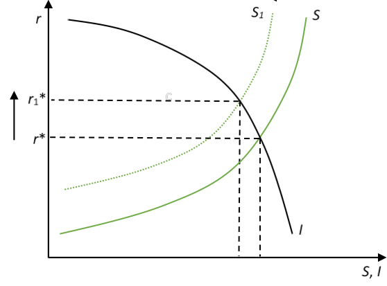
Figure 21.3. Impact of a higher impatience (higher preference for present consumption)
Beyond variables related purely to the decision-making process of private economic units, another factor that influences the natural rate of interest is fiscal policy. When the government deficit spends, it needs to borrow some of the available saving and so enters in competition with demand for funds by investors. This pushes up the natural rate of interest and so discourages private investment (Figure 21.4). The crowding out of private investment reduces economic growth (see Post 12).
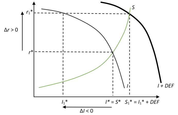
Figure 21.4. Crowding Out Effect
Implications of the Theory
The real theory of interest rate has several implications in terms of the regulation of financial markets, of the role of monetary policy, of the conduct of fiscal policy, and of the promotion of economic growth.
In terms of deregulation, the government should not be involved in setting interest rates. Post 19 and Post 4 have explained that the government is heavily involved in managing interest rates, by setting them or by lowering them. Economists of the real exchange framework see this involvement as a direct cause of financial instability. For example, according to them, the central bank and government-sponsored enterprises have been a major cause of the early-2000s credit boom that translated into a housing boom. The Federal Reserve kept its policy rates too low for too long, Fannie Mae and Freddie Mac (Post 19) helped keep mortgage rates artificially low. Both have encouraged investment well beyond the amount of saving available for housing purpose. Interest rates should be left to be determined by market forces and economic units should be left alone to make a rational calculation to figure out if it is worth investing in a business, in education, among others. Does the marginal benefit outweigh the cost? If not this is not the case, rational economic units will be contented not to own a house or not to go to college because it is not beneficial given the interest rate. They are better off renting and working (or taking leisure time if the wage rate is too low). Markets are there to provide a price signals that is included in the rational decision-making processes, government intervention distorts that signals and so leads economic to make incorrect decisions, which leads to financial crises.
In terms of monetary policy, it would be best for the central bank not to intervene by setting interest rates; instead, the central should target the quantity of reserves to manage the money supply to keep inflation stable. If a central bank decides to manage interest rates, it should set the nominal interest rate in a way that is consistent with the monetary rate of return of non-monetary assets. If the interest rate is set too low, monetary policy will promote a credit boom and inflation, if the interest rate is set too high, monetary policy will generate a recession and deflation. Therefore, it is crucial to have estimate of the natural rate and inflation expectation so that the optimal interest rate (the one that promotes price stability) is found. Central bankers have come to see the management of inflation expectations as a main role of monetary-policy making.
In terms of fiscal policy, a government should avoid deficit spending. While there is some room for fiscal intervention in the short-run, it should be temporary, quick and targeted in order to help put the economy back on its natural path more quickly. There should not be permanent deficits, and a central policy goal of a government should be to aim for a balanced budget. Some economists in that framework have gone as far as promoting a balance-budget amendment to the U.S. constitution so that federal finances works in the same fashion as state finances.
Finally, in terms of economic growth, a government should find ways to promote thriftiness, which will bring down interest rates, encourage investment and so promote economic growth. Rather than working through government programs that artificially lower interest rates, the goal of policymaking should be to change incentives so that individuals make a rational decision to save more. This will allow more resources to be allocated to investment. Financial repression—keeping interest rates artificially low relative to what the market demands—not only promotes financial instability and inflation, but also discourages saving and economic growth. The biggest savers are high-income and high-wealth earners so policies should cater so these individuals, who will then have the incentive to use their wealth and income for the benefit of society by investing in the economy; this is called the trickledown effect. Broader policies, such as tax incentives to save for retirement, can help everybody to save. As explained in Post 19, pension funds work by deferring and reducing tax payments so this may encourage households to save. Thus, the growth of money managers and the financialization of the economy have promoted thriftiness and so increased the availability of funds for investment.
Empirics
The empirical work surrounding the theory studies if nominal interest rates respond to expected inflation/deflation, if fiscal deficits impact the natural interest rate (and so nominal interest rates), and what the level of the natural interest rate is and how it changes over time.
Starting with Irving Fisher, there has been quite an extensive empirical testing of the relationship between interest rates and inflation (expected and actual) in the United States and at the international level. Unfortunately for the theory, the relation has been either inexistent or much weaker than expected. Figure 21.5 shows that, in the United States, there is no relation between inflation measured by the consumer price index (CPI) and interest rates until the mid-1950s. Before 1953, the correlation is zero or negative which is quite striking given that financial markets were highly deregulated prior to the 1930s so savers could have sync interest rates to inflation more easily if that was a major concern. After 1953, the correlation is moderately high especially for short-term interest rates, 0.79 for short-term rates, 0.66 for long-term rates.
Some economists have argued that this change means that financial-market participants have now assimilated Fisher’s framework of analysis, but others note that this change in the relationship between interest rate and inflation has much more to do with a change in monetary policy strategy following the Treasury Accord of 1951. By 1953, the Fed had freed itself completely from any obligations toward ensuring the perfect liquidity of Treasuries by targeting the entire yield curve (see Post 6). By that time, the need to fine tune the economy with policy tools was seen as necessary. Given the growing concerns about inflation and the renewal of Monetarist ideas, the central bank progressively oriented its policy toward fighting inflation. It raised and lowered its policy rates with changes in expected inflation. One of the immediate implications is that the other rates also became more correlated with inflation. Thus, the higher correlation does not reflect the fact that market participants suddenly became more preoccupied with inflation, only the Federal Reserve did.
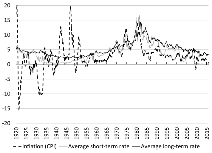
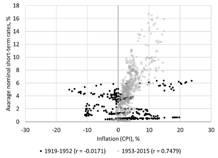
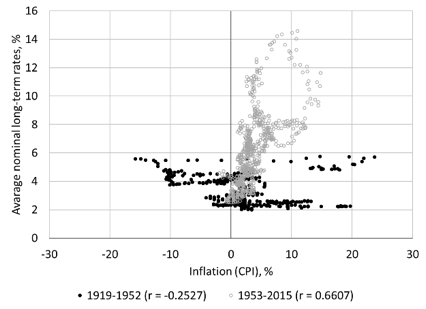
Figure 21.5 Inflation and interest rates
Sources: Board of Governors of the Federal Reserve System (Series H.15), National Bureau of Economic Research (Macrohistory Database), Bureau of Labor Statistics
Empirical tests of the existence or not of a crowding out effect have also been quite extensive and are again inconclusive. Following the theory, one would expect that a higher fiscal deficit would lead to a higher natural rate and so a higher nominal interest rate, and that if the fiscal position moves toward a surplus interest rates would fall. Figure 21.6 shows that, for the United States, a relationship between nominal interest rate and the fiscal position of the government is very weak to inexistent. Figure 21.7 shows a similar lack of relationship if one takes estimates of the natural rate of interest. In the end, for the United States, one cannot conclude that a fiscal deficit will lead to higher interest rates. Post 6 provides an explanation of why: the Federal Reserve System and Treasury work hand in hand to ensure that fiscal operations have no, to very limited, impacts on interest rates. This is a feature of monetarily sovereign countries.
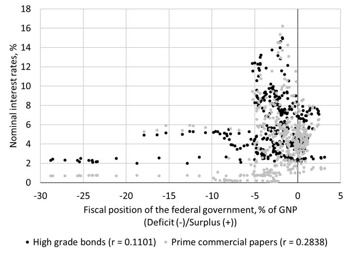
Figure 21.6 Fiscal position and interest rates
Sources: National Bureau of Economic Research (Macrohistory Database, Tables from “The American Business Cycle”), Treasury Bulletin (via FRASER), Bureau of Fiscal Service (Monthly Receipts, Outlays, and Deficit or Surplus, Fiscal Years 1981-2017)
Note: Quarterly data, Q1 1880 to Q4 2016 for fiscal position and commercial papers, Q1 1900 to Q4 2016 for high-grade bonds.
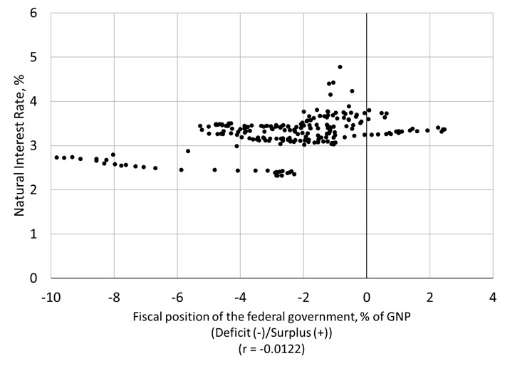
Figure 21.7 Fiscal position and natural interest rate
Sources: National Bureau of Economic Research (Tables from “The American Business Cycle”), Treasury Bulletin (via FRASER), Bureau of Fiscal Service (Monthly Receipts, Outlays, and Deficit or Surplus, Fiscal Years 1981-2017), “Calculating the Natural Rate of Interest: A Comparison of Two Alternative Approaches” by Thomas A. Lubik and Christian Matthew.
A final empirical endeavor of the theory has been to measure the natural interest rate. This variable is not observable so it must be estimated out of supply conditions in the economic system, such as productivity of capital, the natural growth rate of the economy, demographic trends, among others. There is a debate among economists following that framework about the reliability of available estimates and their usefulness for policy purpose. Estimates are model-dependent (depending on the hypotheses made the estimate can be significantly different) and time-dependent (the natural rate changes over time) and there is large uncertainty around the mean. These econometric difficulties are similar to the ones applying to measures of the natural growth rate and the natural unemployment rate. Still economists following that framework are hopeful that better model specifications, better estimation techniques and refined data will bring a reliable measure of the natural rate of interest.
Monetary Theory of Interest Rates: Monetary Conditions and Liquidity Preference
Economists using the monetary production economy framework do not find the previous theory satisfying for multiple theoretical and empirical reasons. The empirical aspects have been presented above. In theoretical terms, one can reduce the problem to two issues, one is the over-reliance on the role of relative prices and substitution effects, and the other is the lack of recognition of the central role of monetary aspects in decision-making processes. Economic units are deeply concerned about staying liquid and judge economic results in nominal terms, as such, the interest rate is impacted by these concerns. In the 1930s, John Maynard Keynes proposed a theory of interest rate that addresses these issues.
Substitution Effect vs. Income Effect
The loanable funds theory relies on the smooth working of relative price mechanisms to reach a stable equilibrium; if there is a surplus relative price falls, if there is a shortage relative price rises. Production involves two inputs, labor and capital, and firms are indifferent between the two inputs so they use the cheapest. The price of labor is the real wage (w), the price of capital is the real interest rate (r), and so the relative price of capital is r/w. In the loanable theory, a fall in r encourages investment because r/w falls and so firms substitute capital for labor. Similarly, the fiscal impact of deficits is only judged from the point of view of its substitution effect: a deficit raises r and so r/w, which encourages firms to substitute labor for capital, investment falls.
Two issues come up with this logic. First, there has been a long recognition that there is no reason to assume that relative-price adjustments work in a smooth fashion (rapid changes in relative prices create instability) or bring a market to equilibrium (the equilibrium is unstable). In general, a downward slopping investment curve (or demand curve more generally) does not apply, and a decrease in r/w can be associated with a decline, a rise or no change in investment. The “Cambridge Controversy”—a theoretical debate that occurred in the 1960s between scholars located Cambridge, MA, USA and Cambridge in the UK—is the latest example of such conclusion. Thus, one cannot rely on relative price adjustments to reach an equilibrium. This criticism can also be applied to what is presented below (and anytime there is a supply-demand graph).
Another issue is that a fiscal stimulus, via deficit spending, also generates an income effect. For example, the Kalecki equation of profit presented in Post 11 shows that:
U = I + DEF + NX
With U aggregate profit, I private domestic investment, DEF the government deficit, and NX net exports.
When government deficit spends, the private sector receives an injection of income—firms sale more and so record higher profits. This, in turn, encourages investment because higher profits boost the confidence of entrepreneurs and their profit expectations. Thus, assuming that the substitution effect is valid, there are two impacts from a government deficit (Y is aggregate income):

The problem becomes to figure out which of the two effects dominates. Economists following the monetary production economy framework argue the substitution effect is empirically marginal if not falsified, in addition to being theoretically unsound. Firms do not care much about the cost of credit when they invest, expectations of future cash flows dominate the decision to invest.
The inclusion of income effects has another vexing implication for the loanable funds theory, because the saving and investment curves are no longer independent. At the aggregate level, the amount of saving depends on the level of income, but that level of income depends on the level of spending such as investment. Thus, there is no unique natural rate of interest rate but an infinity of them, because the natural rate depends on the level of economic activity, so it is influenced by demand conditions and not merely supply conditions.
Again, the Kalecki equation of profit makes that clear; if investment goes up so does profit (the saving of firms), and if firms earn more, they employ more individuals who in turn earn an income and so can save. The ultimate impact on the natural interest rate is undetermined because higher aggregate investment leads to higher aggregate saving. A shift in the demand curve (via investment or government deficit) can lead to higher, lower, or unchanged r* depending on the slope of each curve and depending the size of the shift in the saving curve. Figure 21.8 shows a case where the natural rate is unchanged.
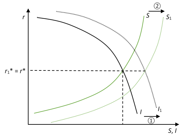
Figure 21.8. Income effect in the loanable funds market.
Liquidity Preference Theory of Interest Rate
Given all these issues, economists working in the monetary production economy framework have used an alternative theory of interest rate that was first presented by Keynes. Capitalist economies are monetary economies. Similar to a barter economy that uses monetary instruments, such an economy uses monetary assets to transact, but, contrary to a barter economy, monetary outcomes influence incentives and decisions. Economic units compete among each other and judge results in monetary terms not in real terms because all contracts and obligations are written in nominal terms nor real terms (Post 12). Such an economy is subject to uncertainty, that is, nobody knows what the future hold in terms of monetary outcomes, and probabilities are either inexistent or not a reliable means to judge the future. Such an economy is driven by demand conditions (expected sales of output), and no market exists to smooth aggregate income over time and to make intertemporal decisions about real income. Indeed, current spending determines current income and if spending fall (saving rises) income falls (Post 12) because there is no certainty if, nor when, that current saving will be consumed in the future. Saving is not equivalent to future consumption and so a decline in present consumption (a rise in saving) discourages investment, which lowers aggregate income even further.
Given this institutional context, economic units care about financial solvency, so they care about monetary profitability and liquidity in addition to purchasing power concerns. Liquidity helps to stay solvent but limit profitability, and economic unit aim at finding the proper mix of assets in their balance sheet given their liquidity preference.
From this starting point, Keynes makes four points about the lack of substitution among assets, about what the interest rate rewards, about the overwhelming impact of the stock of financial instruments on the interest rate, and about the importance of capital gains in the calculation of the rate of return.
First, the liquidity of a balance sheet impacts solvency so liquidity is a central concern of economic units. Economic units are not indifferent between holding liquid assets and illiquid assets. In normal times, when the monetary system works properly, only liquid assets provide a reliable means to store value through time so there is no gross substitution among all assets. Economic units prefer to hold liquid assets. If an asset is less liquid, holding it carries some risk and so economic units will require a higher rate of return that reflects their concerns and preference for liquidity. The higher their preference for liquidity, the higher the reward they will demand to buy an illiquid asset.
Second, if someone earns $100 and decides to save $20 in cash, cash does not provide any interest. Thus, the interest rate is not a reward for merely saving some income; it is a reward for moving the asset portfolio into illiquid positions. For example, say Mr. X earns $100 every month and has to decide if he should save some of it. According to Keynes, the interest rate is not playing much of any role in that decision; the consumption-saving decision is mostly based on habits of consumption and uncertainty about the future (if X expects to be unemployed in the near future he saves more now); the marginal propensity to consume (mpc) determines the split of income. Where the interest rate plays a role is in the decision about the distribution of assets in the balance sheet and how satisfied economic units are with that distribution. Say that over the years, X has saved $10,000 in a checking account and the checking account is his only asset, how should X place that $10,000? Should X hoard all of it in a checking account, should X buy stocks or bonds? Should X buy a home to rent it and/or for speculative purposes? Why proportion of the $10,000 should stay in the checking account? The nominal rate of return on each asset helps X decide which assets is worth holding given his liquidity preference (Figure 21.9).
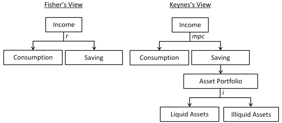
Figure 21.9. The role of the interest rate in two theories
Third, the emphasis on flow variables in the determination of interest rates is misguided. Stock variables play an overwhelming role on the price of assets because stocks are much larger than flows. Flow variables ∆S (net addition to an outstanding amount; think of water flowing into a bathtub) adds to stock variables S outstanding (the amount of water in the bathtub):
St = St-1 + ∆St
In the loanable funds theory, the net increase in the demand for securities is the amount of saving, while the net addition to the stock of securities is the offering made by firms that want to invest. For Keynes, these net increases in supply and demand are too small of a magnitude of have much of an impact on the price of securities and so the interest rate; instead, it is the outstanding quantity of securities and the demand for that outstanding quantity (the willingness to hold these securities) that matters to set interest rates. Do people want to hoard the monetary assets they have? That is, is the demand for monetary instrument (willingness to hoard) equal to the available quantity of monetary instruments? (Figure 21.10). Put in accounting terms, the interest rate is determined by balance sheet considerations (willingness to hold the assets owned) not by income considerations (willingness to save some income).

Figure 21.10. Flow equilibrium (loanable funds theory) versus stock equilibrium (liquidity preference theory)
Some economists tried for decades to show that a flow analysis leads to the same equilibrium interest rate as a stock analysis. However, this conclusion holds only under perfect foresight, or rational expectations, which is not compatible with the framework used by Keynes and economists operating in the monetary production economy framework. In case of perfect foresight, liquidity concerns are no longer important and one is back to the real exchange economy framework.
Fourth, contrary to the Fisherian approach and the Efficient Market Hypothesis, one cannot consider that the monetary return on an asset (financial or nonfinancial) solely depends on income. To maintain their liquidity and to boost nominal returns, economic units do care about the direction of the price of a securities, and so care about the future nominal interest rates when making portfolio decisions. If expectations of a rise in interest rates are such that economic units think that capital losses will more than offset income gains, they will stay in liquid assets even if the current interest rate on illiquid assets is positive. This is situation is called a liquidity trap.
Money Rules the Roost
Similar to Fisher, Keynes argues that economic units will choose to hold whatever asset pays the most and they will arbitrage among assets. This arbitrage will continue until all rates of return are equal. Differently from Fisher, Keynes argues that it is the rate of return on financial instruments—the interest rate—that is the anchor of the system. The rate of return on financial instruments sets the minimum monetary rate of return that non-financial instruments must achieve. Again, at the aggregate level, one can reduce the arbitrage to one between capital equipment and monetary instrument (Figure 21.11).
The rate of return on capital equipment is called the marginal efficiency of capital (mek) and the rate of return on lending monetary instruments is the interest rate i. If mek > i, firms issue debts to obtain monetary instruments and use the proceeds to buy capital assets. If they buy new capital assets, aggregate investment occurs. As more machines are produced, the mek falls because it becomes more difficult to sell output at a given price as markets become saturated (there is only a limited number of customers for a given product). If mek < i, firms decrease their investment level. The problem becomes to figure out what determines the interest rate.

Figure 21.11 Adjustment mechanism in the monetary production economy framework
Liquidity Preference and Rates of Return
The expected monetary rate of return z of asset j depends on the following factor:
zj = qj – cj + ℓj + aj
That is, the expected rate of return on any asset depends:
- Positively on the yield q, the expected income earned from holding the asset. If that asset is a non-financial asset, q represents the rate of return earned from the sale of production. If it is a financial asset, q is earned from monetary payments received in the form of interest payments or dividends.
- Negatively on the carrying cost c, the expected expenses incurred to take position in an asset. These expenses include maintenance expenses, insurance, interest payments if debts are issued to finance asset positions, among others.
- Positively on the expected capital gain (a > 0) or loss (a < 0) from selling the asset.
- Positively on the liquidity premium ℓ, the reward to pay on illiquid assets to incentivize someone to give up a liquid asset. The higher the perceived liquidity of an asset, the higher ℓ. Note that ℓj is not rewarded directly by asset j; it is not earned by holding asset j (qj) nor is it earned by selling asset j (aj). It is a reward obtained on asset j by giving it up for another asset that is less liquid. Put differently, the more asset j is liquid, the more one is able to bid down the price of other assets to buy them with asset j. For example, monetary instruments do not pay any interest and always trade at parity but they can be used to bid down the price of other financial instruments, which raises the interest rate.
This nominal rate of return can be adjusted via q to account for inflation, but expected inflation and income are not the only thing that matter and, as explained in Post 20, economic units may pay much more attention to staying liquid and speculating. Depending on the assets, some of the component are more important:
- Asset 1: Output-producing nonfinancial assets (capital equipment). These assets are illiquid so the reward obtained from parting with them can be considered nil (ℓ1 = 0%); they cannot be used to bid down the price of other assets. The rate of return is influenced by expected profit earned from selling the output produced by the equipment, and the expected capital gain/loss from reselling the asset: z1 = q1 – c1 + a1.
- Asset 2: Unproductive nonfinancial assets (commodities): These assets are mostly illiquid because the price of commodities is highly volatile (ℓ2 = 0%), and they do not directly produce any output that can be sold (q2 = 0%). However, they can provide a return from reselling them at a higher price (a2). While they are held, one must cover some expenses for stocking them, insuring them, among others (c2). The rate of return is: z2 = a2 – c2.
- Asset 3: Financial instruments other than monetary instruments: There may or may not be a more or less active market to trade them so the degree of liquidity will vary from illiquid (mortgage notes) to very liquid (Treasuries). The rate of return on financial instruments, the interest rate, is z3 (= i) = q3 – c3 + ℓ3 + a3.
- Asset 4: Monetary instruments: They are perfectly liquid so ℓ4 is the highest of all assets, that is, bearers want to be reward to part with monetary instruments. Given that they are perfectly liquid they always trade at face value (a4 = 0%). They also do not provide any income (q4 = 0%) and the carrying cost is marginal (c4 = 0%) unless monetary instruments were obtained through credit. The rate of return is: z4 = ℓ4. ℓ 4 represents the minimum rate of return that must be provided by less liquid assets to incentivize to bearers of monetary instruments to buy them.
If economic units become pessimistic, their liquidity preference goes up and they will ask for a higher reward to go illiquid: ℓ4 and ℓ3 go up. This means that the price of less liquid asset falls—and so the rate of return they provide rises—, and it has to fall enough to give an incentive to holder of liquid assets to part with them (Figure 21.12).
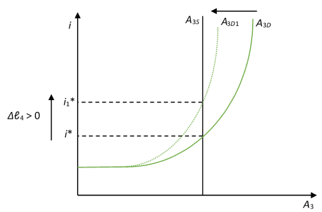
Figure 21.12 Effect of an increase in liquidity preference on the demand of less liquid assets
To show the central role that monetary considerations play in the determination of the interest rate, the effect of a change in liquidity preference is usually represented in terms of the demand for monetary instruments. An increase in the demand for illiquid assets is equivalent to a decrease in the demand for liquid assets. As such, the demand for monetary instruments moves inversely with the interest rate paid by financial instruments; a higher interest rate leads to a lower demand for monetary instruments (a lower willingness to hoard the outstanding stock of monetary instruments). The demand for monetary instruments flattens as the interest rate falls because of the liquidity trap. A higher liquidity preference increases the willingness to hoard the exiting stock of monetary instruments at any given interest rate, so the equilibrium interest rate rises (Figure 21.13).
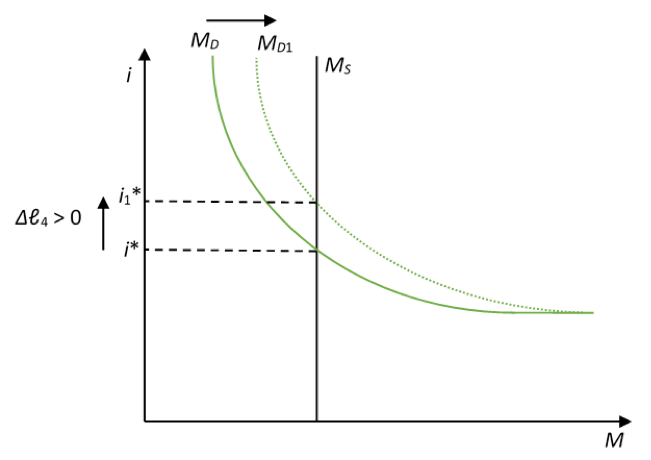
Figure 21.13. Impact of liquidity preference on the interest rate on an asset
Figure 21.13 assumes that neither the central bank nor private banks purchase illiquid assets from those who want to sell, if they do, the supply of monetary instruments rises to accommodate exactly the desire for additional monetary instruments, and the interest rate stays unchanged. The supply of monetary instruments is horizontal in that case.
Implications of the Theory
The main implications are that monetary conditions influence the nominal interest rate through more direct channels than expected inflation and lower the interest rate, that the crowding out effect is not automatic, that lender of last resort policies are crucial and monetary policy should be about targeting interest rates, that supply-side factors have only an indirect and limited impact on interest rates, that promoting thriftiness discourages investment and may encourage speculation.
First, monetary conditions (quantity of liquid assets, policy rate of the central bank and liquidity preference) play a central role in determining the nominal interest rate and this influence is direct, it does not go through inflation. The immediate impact of a change in monetary conditions is not to change output prices (inflation) but to change financial-asset prices (interest rates). Output prices are determined by costs and the state of the economy (Post 11). In addition, contrary to the real theory of interest rates, the impact of a loosening in monetary conditions is to lower interest rates. If the supply of monetary instruments goes up, or if the supply of reserves goes up, or if the interest-rate target falls, or if the confidence of economic units increases, then the demand for illiquid assets rises and the demand for liquid asset falls; economic units want to have a less liquid balance sheet. As they buy less liquid financial instruments, the interest rate falls. Given that monetary conditions are paramount to determine nominal interest rates, and given that the central bank control some key interest rates on a daily basis (Post 4), daily monetary policy has an overwhelming influence on nominal interest rates.
Second, given the centrality of monetary conditions, an increase in the demand for funds—for investment purposes or to finance a deficit—does not have to lead to a rise in interest rates. It depends on how monetary conditions adapt to the increased need for funds. If liquidity preference falls enough, economic units with monetary assets are more willing to part with them and the interest rate does not change. If the supply of monetary instruments rises enough, the impact on the interest rate is nil. Thus, the crowding out effect is not automatic. Of course, if the interest rate on a financial instrument is fully or partially control, like the interest rate on federal funds debts or the interest rate on Treasuries, the fiscal position will have no or limited influence on interest rates. Only changes in the interest rate target (iT) will have a significant impact (Post 4 and Post 6) (Figure 21.14).
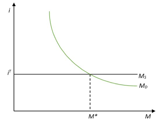
Figure 21.14. Interest rate targeting and liquidity preference
Third, it is essential to have an economic unit that is willing to help stabilize interest rates. When views of the future change for the worse, interest rates rise sharply because economic units try to sell illiquid assets and to hoard more liquid assets. This volatility occurs because those who seek to change the composition of their balance sheet cannot change the supply of both assets. Banks cannot create reserves, households and nonfinancial firms cannot create the monetary instruments they desire to hoard. A sharp rise in interest rates has an adverse impact, on the net worth of economic units that own a high proportion of less liquid long term assets (duration is larger for long-term assets, see Post 20), on the ability to refinance existing debts (Post 7), on the ability to service debts with a variable interest rate. To counter the fetish for liquidity that emerges in period of heightened uncertainty, an economic unit should stand ready to provide liquid assets to satisfy that fetish. A central bank should respond to the willingness of other economic units to increase their proportion of liquid assets in their portfolio. It can do so by being ready to buy less liquid assets on demand, or to provide credit on demand against such less liquid assets. The central bank should act as lender of last resort. More broadly, the central bank should be involved in smoothing the variability of interest rates on a daily basis; monetary policy is about setting at least one interest rate, it is not about setting the amount of reserves (Post 5).
Fourth, the emphasis on productivity, time preference and other supply-side aspects is unwarranted. What matters for the rate of return on capital equipment is the ability to sale the output (q) not merely the ability to produce it (marginal product), and there is nothing that ensures that what is produced will be sold even if prices fall. Say’s law does not apply in a monetary economy and debt deflation prevents a smooth clearing of market surpluses (Post 11). In addition, capital-gain expectations play a crucial role in determining rates of return, this is all the more so that the asset is marketable. In this case, market participants may not want to raise the interest rate in sync with inflation because, while raising interest rate may protect income against inflation, capital losses may materialize.
Fifth, promoting a liquid markets and giving incentive to put wealth into less liquid form assets may not promote aggregate investment. Economic units arbitrage among all assets and buy those that provide the highest return over the holding period they prefer. Instead of buying new capital equipment—investing—they may buy old capital equipment or they may buy commodities and financial assets. Post 20 explained that financial-market participants tend to have a short holding period and to have a speculative mentality (bet on price direction) rather than an investment mentality (buy and hold asset to patiently wait for income). Nonfinancial companies may also prefer to buy financial assets instead of nonfinancial assets, and this has been a trend in their balance sheet (Post 7). Post 19 showed that the stock market is not a net contributor of funds and that nonfinancial companies have been buying back their stocks to boost their prices. Thus, promoting thriftiness not only discourages investment but also may promote speculation if liquid financial instruments are available.
Empirics
Empirical evidence clearly shows that interest rates on long-term and short-term securities move in sync with monetary policy decisions, this is especially so for short-term rates that have a correlation coefficient of 0.99 with the federal funds rate. Long-term rates have “only” a correlation coefficient of 0.88, which leaves some influence for other factors, such as expected inflation, expected fiscal position, concerns about credit risk, among others (Figure 21.15). The impact of monetary policy on long-term rates will be all the stronger that financial-market participants do not expect the policy to be reversed for a while, that is, if they believe that the central bank will keep doing the same thing (rising, lowering, or not changing its policy rates) for a while. The following post on interest-rate structure will develop that point.
So nominal interest rates are low because the central bank sets a low policy rate and they will stay low as long as the central bank does not raise the rate, even if inflation expectations rise, even if the government deficit spends a lot, even if the natural rate of interest rises. Interest rates will stay low even if liquidity preference increases as long as the central bank is willing to intervene enough to stabilize rates it does not normally stabilize directly. An extreme version of this influence of monetary policy is when the central bank decides to set both short-term rates and long-term rates, like it did for Treasuries during World War Two (Post 6).
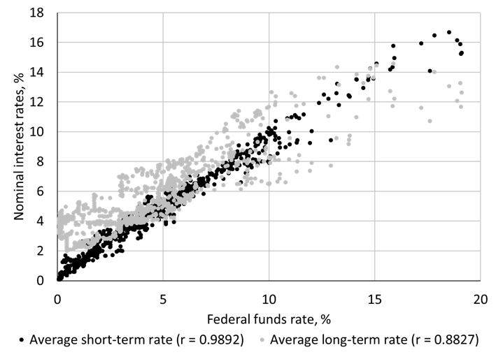
Figure 21.15 Monetary policy and interest rates
Sources: National Bureau of Economic Research (Macrohistory Database)
Note: Monthly data from January 1919 to December 2015
The fact that monetary policy plays a central role in determining the interest rate does not mean that the central bank fully control all interest rates. As the correlation coefficient above suggests, there is some role for other factors to play in the determination of long-term interest rates. For example, Figure 21.16 shows that Quantitative Easing, that resulted in large injection of reserves (Post 4) and an increase in the money supply (Chapter 5), did not lead to a fall in long-term Treasuries. In fact, long-term Treasuries rates had a tendency to rise during the period of Quantitative Easing and to fall once it ended. The central bank did not do enough to control long-term rates. Although it bought a large quantity of them, it did not do so with a specific target rate in mind like during World War Two. Targeting an interest rate involves buying, or selling, whatever dollar amount is necessary at a price consistent with the interest rate target (Post 4). Quantitative Easing involved buying a predetermined monthly dollar amount ($75 billion worth of Treasuries each month for QE2, $40 billion worth of mortgage-backed securities each month for QE3) at whatever price the market would bear.
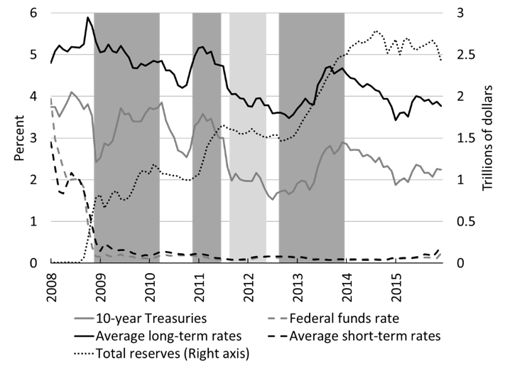
Figure 21. 16. Quantitative Easing (Dark-grey bars), Operation Twist (Light-grey bars), Federal funds rate and interest rates
Source: Board of Governors of the Federal Reserve System (Series H. 15) and Wikipedia (History of Federal Open Market Committee actions)
Note: Quantitative Easing (formally know has Large-Scale Asset Purchase Program) involved buying and holding large quantities long-term securities, which resulted in trillions of dollars of injections of reserves. Operation Twist involved changing the composition of the balance sheet of the central bank by simultaneously selling short-term Treasuries and buying long-term Treasuries, with the goal of lowering long-term rates while avoiding any net injection of reserves.
TO GO FURTHER: LIQUIDITY TRAP AND THE SQUARE RULE
The liquidity trap was introduced by Keynes in the following way:
[E]very fall in i reduces the current earnings from illiquidity, which are available as a sort of insurance premium to offset the risk of loss on capital account, by an amount equal to the difference between the squares of the old rate of interest and the new. For example, if the rate of interest on a long-term debt is 4 per cent., it is preferable to sacrifice liquidity unless on balance of probabilities it is feared that the long-term rate of interest may rise faster than by 4 per cent. of itself per annum, i.e. by an amount greater than 0.16 per cent. per annum. (Keynes 1936a: 202)
This “square rule” implies that someone who expects the level of the rate of interest to go up by more than its square should increase his preference for monetary instruments. To see this more clearly, assume that an individual can choose between keeping his monetary assets or buying a perpetual bond and selling it after one coupon period. The expected nominal return obtained on the perpetual is the sum the coupon and expected capital gain/loss:
R = C + E(ΔP)
Which, knowing that the fair price of a perpetual bond is P = C/i, is equal to:

Consistent with Keynes’s liquidity preference theory in which money “rules the roost,” one placement strategy involves determining what change in the nominal bond rate is expected to lead to a nil nominal return (E(R) = 0):

Thus, for a perpetual bond, the short-term breakeven point (the point at which coupon offsets capital loss so that the dollar return is zero) is reached when the level of the rate of interest varies by its square (when it grows at the level of itself). Therefore, if i is expected to increase and E(Δi) < i2, the short-term holding of a perpetual bond provides a net dollar gain. The capital loss is expected to be inferior to the coupon and the individual should lower his demand for monetary instruments (should buy the bond).
Keynes called the case E(Δi) > i2 a liquidity trap. In this case, the central bank loses its capacity to influence nominal long-term rates, because the demand for monetary instruments rises infinitely from the prevailing interest rate; the demand for monetary instruments becomes horizontal (see Figure 21.13). Keynes stated that this kind of condition is rare, if ever observed. However, the previous condition was obtained by assuming that the targeted dollar return over the period was zero and by only looking at placement strategies over one coupon period.
If one of these strict conditions is removed, the liquidity trap has much more chance to appear. For example, it is highly probable that financial-market participants have a positive rate of return in mind that makes them indifferent. Let us say that a person, at time 0, could buy a bond for a sum M0. In addition, let us assume that this person has a targeted nominal sum, MT, that he would like to receive after one coupon period. His targeted yield over the coupon period is zT = MT/M0 – 1, which generates a targeted nominal return of zTM0 over the coupon period. A person, therefore, will be indifferent between bond and money if:

Thus, the expected change in the market rate that leaves the person indifferent is:

The higher the targeted sum at the end of the coupon period, the smaller the change in interest rates tolerated will be before parting with a perpetual bond. Given that S0 is the current fair price P (the person holds only one bond) and that FV is the par value of a bond so that C = cFV, and c is the coupon rate, we have the following indifference condition for a perpetual bond (p = P/FV):

The higher the targeted return relative to the coupon rate, and the higher the fair price relative to its par value, the smaller the change in interest rate tolerated by actual and potential financial-market participants, and the more the liquidity trap has a chance to emerge. For a high enough targeted yield, an expected decline in the interest rate is necessary not to affect adversely financial positions.
While Keynes presents the liquidity trap with perpetual bonds, the logic of the argument can be generalized to all long-term financial instruments. The point is that long-term interest rate, i, may become insensitive to monetary policy when policy rates become low and are expected to rise again soon.


One response to “Money and Banking Post 21: The Interest Rate”