
By Eric Tymoigne
We are done with the study of banking operations. The next step is to incorporate them into the analysis of macroeconomic issues and this post begins on such topic by focusing on inflation. When inflation is mentioned, it is usually in relation to the cost of buying newly produced goods and services for consumption purpose. Another type of inflation concerns asset prices, i.e. the price of non-producible commodities and old producible commodities. This post does not study asset-price inflation, which concerns theories of interest rate.
Theories of Output Prices
There are two broad ways to categorize existing explanations of inflation (and deflation); monetary explanations and real explanations (“real” means related to production). Below are two popular theories based on such categorization.
The Quantity Theory of Money (QTM): Monetary View of Inflation
The QTM starts with the identity MV ≡ PQ with M the money supply, V the velocity of money (the speed at which the money supply circulates to complete all necessary transactions), P the price level, and Q the quantity of output. The identity is a tautology, it just says that the amount of transactions on goods and services (PQ) is equal the amount of financial transactions needed to complete those transactions. To get a theory of output price (the QTM), one must make some assumptions about each variable and make a causal argument. The QTM assumes that:
- H1: M is constant (or grows at a constant rate) and is controlled by the central bank through a money multiplier
- H2: V is constant (habits of payments are stable)
- H3: Q is constant at its full employment level (Qfe) or grows at its constant “natural” rate (gQfe). Supply conditions (productive capacities) are supposed to be independent from the demand conditions (spending on goods and services).
Given this set of hypotheses we have:
P = MV/Qfe
Or, in terms of growth rate (V is constant so its growth rate is zero):
gP = gM – gQfe
If the money supply grows faster than the natural rate of economic growth, there is some inflation (gP > 0). If gM = 2% and gQfe = 1% then gP = 1%. If the central bank increases the growth rate of the money supply, inflation rises by the same percentage points while the growth rate of production is unchanged. Inflation has monetary origins.
The economic logic is the following in terms of price level. First, suppose some money falls into the hands of economic units. How? Milton Friedman is famous for arguing that economists do not need to care about how the money supply enters the economy; one can merely assumes that it falls from a helicopter. Following H1, one may say that the central bank injects reserves, which leads to a large increase in the amount of bank credit.
So now economic units have a bunch more monetary instruments. They could save them but H2 implies that economic units have hoarded everything they wanted to hoard so economic units rush to stores to spend. Given that the economy is at full employment, the only way the economic system can adjust to the large increase in the demand for goods and services is through an increase in prices. Money is “neutral,” it does not impact production.
The main policy implication is that central banks are best suited to tackle inflationary problems, while productive issues are best left to relative price adjustments via market mechanisms. The central bank can manage output prices by targeting the quantity (growth rate) of reserves and by setting the reserve requirement ratio. This will constrain the quantity (growth rate) of money supply and set a specific price level (inflation). Controlling inflation is an easy job, a central bank just needs to decide what its inflation target is (gPT) and to determine what the natural growth rate of the economy is (gQfe). If, for example, a central bank has an inflation target of gPT = 2% and the natural growth rate of the economy is gQfe = 3%, the growth rate of the money supply should be gM = 5%. Assuming a stable multiplier, this means that the growth rate of reserves should be 5%.
This argument has been extended to a central bank that targets an interest rate. Most central bankers now recognize that monetary stimulus is not neutral in the short-term, hence the ability to fine-tune—i.e. to make sure the economy is not too hot (inflation) nor too cold (unemployment)—the economy through an interest-rate policy. However, in the medium to long-run, the neutrality of money is argued to prevail, hence the importance of inflation targeting. Central bankers can use that to guide their short-run policy. Central banks should determine a reference value for the growth of money supply (gM*). This value should be consistent with the inflation target (gPT), the prevailing natural growth rate, and the existing trend of velocity (gV):
gM* = gPT + gQfe – gV
If gM > gM*, a central bank is too lax (i.e., its interest rate target should be higher) and inflation will be above target in the medium term.
There are several issues with that approach that relate to the hypotheses made to reach the conclusion and to the causality at play:
- The money supply is not controlled in anyways by the central bank. Not only does the money multiplier theory not apply, but also the growth of the money supply is driven primarily by the demand for bank credit by private economic units (banks cannot force feed credit to economic units) and by government spending and taxing.
- Interest-rate targeting has only a remote and uncertain effect on the growth of the money supply, even more so on inflation.
- The economy is rarely at full employment so if the demand for goods and services increases the supply of goods and services increases.
- Measuring the natural growth rate of the economy is actually difficult. More importantly, the demand for goods and services and supply of goods and services are not independent factors. Demand matters even in the “long run.” Greenspan put it nicely during an FOMC meeting:
“Let me just say very simply – this is really a repetition of what I’ve been saying in the past – that we have all been brought up to a greater or lesser extent on the presumption that the supply side is a very stable force. […] In my judgment our models fail to account appropriately for the interaction between the supply side and the demand side largely because historically it has not been necessary for them to do so.” (Greenspan, FOMC meeting, October 1999, pages 46–47)
- In terms of basic empirical evidence, the strong correlation between money supply and price that one should expect does not exist even in the long-run (Figures 1 and 2). While correlation improves as the length of time increases (one-year correlation is 0.55, five-year correlation is 0.67, ten-year correlation is 0.71), the correlation is weaker than what the theory suggests.
- The fact that inflation and money supply growth are positively correlated does not tell us the direction of causality. One may doubt that the causality goes from M to P given the strong assumptions required for that to be the case. The next section will develop this point.
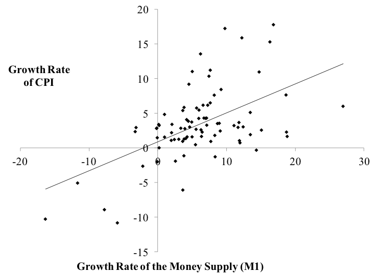
Figure 1. Annual Growth Rate of CPI and of the Money Supply
Sources: BLS, Federal Reserve
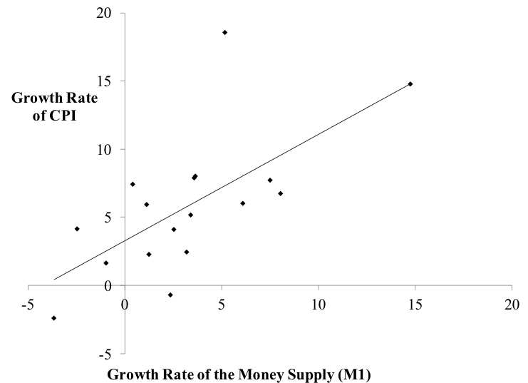
Figure 2. Five-year growth rate of CPI and of the money supply
Sources: BLS, Federal Reserve
Income distribution and inflation
Another theory of the price level starts with an identity grounded in macroeconomic accounting:
PQ ≡ W + U
This is the income approach to GDP. It says that nominal GDP (PQ) is the sum of all incomes. For simplicity, there are only two incomes: wage bill (W) and gross profit (U). All of them are measured before tax. Divide by Q on each side:
P ≡ W/Q + U/Q
W is equal to the product of the average nominal wage rate (w) and the number of hours of labor (L): W = wL (for example, if w is $5 per hour and L is equal to 10 hours, then W is equal to $50). Thus:
P ≡ wL/Q + U/Q
Q/L is the quantity of output per labor hour, the average productivity of labor (APL):
P ≡ w/APL + U/Q
w/APL is the unit cost of labor. U/Q is a macroeconomic mark-up over the labor cost. To get to a theory, the following assumptions are made:
- H1: the economy is usually not at full employment and Q (and economic growth) changes in function of expected aggregate demand (this is Keynes’s theory of effective demand).
- H2: w is set in a bargaining process that depends on the relative power of wage-earners (the conflict claim theory of distribution underlies this hypothesis)
- H3: U, the nominal level of aggregate profit, depends on aggregate demand (Kalecki’s theory of profit underlies this hypothesis, see below)
- H4: APL moves in function of the needs of the economy and the state of the economy, it is procyclical to the state of aggregate demand for goods and services. In general, in periods of labor-time scarcity gAPL goes up and, during an economic slowdown, gAPL goes down before employees are laid off.
Thus:
P = w/APL + U/Q
The price level changes with changes in the unit cost of labor and the size of the macroeconomic mark up. In terms of rates of growth:
gp ≈ (gw – gAPL)sW + (gU – gQ)sU
With sW and sU the shares of wages and profit in national income (sW + sU = 1). Thus, inflation has two sources:
- Cost-push inflation: the growth rate of the unit labor cost of labor (gw – gAPL) depends on how fast nominal wage grows on average relative to the growth rate of the average productivity of labor. The correlation between the unit cost of labor and inflation is very strong both in the “short-run” (0.82 for yearly growth rates) and “long-run” (0.93 for five-year growth rates) (Figure 3).
- Demand-pull inflation: U follows Kalecki’s equation of profit which states that the level of profit in the economy is a function of aggregate demand. Thus, the term, gU – gQ represents the pressures of aggregate demand on the economy; it is an output gap. If gU (the growth of aggregate demand) goes up and gQ (the growth of aggregate supply) is unchanged, then gP rises given everything else. However, to assume that gQ is constant is not acceptable unless the economy is at full employment. Usually, a positive shock on aggregate demand growth leads to a positive increase in aggregate supply growth because the rate of utilization of productive capacities is below one even in “the long run.”
Note that the money supply is absent from this equation. The money supply does not directly affect output prices. Spending may impact inflation but it depends on the state of the economy.
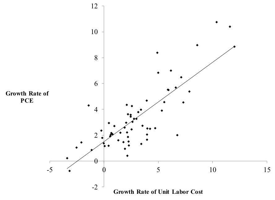
Figure 3. Annual Growth Rate of Unit Cost of Labor and Growth Rate of PCE
Source: BEA, Federal Reserve
Note that the growth rate of wage is by itself not as relevant. It is its relation to the growth rate of the average productivity of labor that matters. Time-series data provides another insight into the role of the unit cost of labor (Figure 4). From the mid 1960s to the early 1980s, unit cost of labor was a main source of high inflation. Nominal wage growth outpaced productivity growth, both grew on average. The former was in the 5-10% range whereas the latter was mostly in the 0-5% range. In the late 1960s, workers were able to outpace productivity growth because of their strength in wage bargaining due to low unemployment and strong unions. The 1970s oil shocks boosted inflation and workers tried to maintain their real wage (they failed) by demanding an increase in nominal wages. This further reinforced inflation because productivity could not keep up with wage demands. The internationalization of labor and the decline in the power of unions have tamed the ability of wages to outpace productivity even in periods of long economic growth.
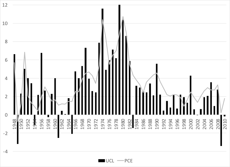
Figure 4. Unit cost of labor growth rate and inflation, Percent
Source: BEA, BLS
When combined with the explanation of monetary creation presented in Post 10, this theory of inflation provides an explanation of the correlation between price and money supply that involves a reversed causality compared to the QTM. Higher costs of production and higher demand pressures push up the price of goods and services, which increases the size of the bank advances that economic units request: higher P (gP) leads to higher M (gM).
A broader point is that the growth of the money supply is not by itself inflationary because money supply grows with the needs of the economic system, economic units are not suddenly allocated bags of money supply with which they do not know what to do:
- Firms request bank credit to start production (pay workers, buy raw material) and repay their bank debts (which destroys money supply) once production is sold: money supply moves in part with the need of the productive system
- Federal government spending (that injects money supply) and taxing (that destroys money supply) move automatically in a countercyclical fashion to tame inflationary pressures (“automatic stabilizers”): during an expansion (a recession), the growth rate of government spending falls (rises) and the growth rate of taxes rise (falls). In the US, most of the automatic stabilizer effect comes from wild fluctuations in the growth rate of taxes (in a recession economic units have less income so they are taxed less) (Figure 5).
So the money supply is not something that falls from the sky, its injection and destruction in relation to the production process must be explained and the debts incurred by monetary creation must be included in the analysis. If the economy is growing, money supply grows, if economic units do not want to hold monetary instruments they may just use them accelerate the repayment of their bank debts.
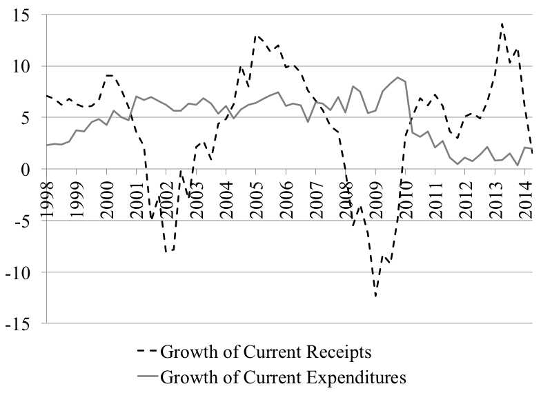
Figure 5. Automatic Stabilizers.
Source: BEA.
In terms of policy, the theory means that inflation is managed best by buffer-stock policies and income policies, or a combination of both such as a job-guarantee program. Monetary policy does not have much direct impact on inflation, and an increase in interest rates can contribute to inflation through the cost and demand impacts of higher interest rates (see below). The role of a central bank is to preserve financial stability through the provision of a stable low cost refinancing source and through regulation.
To go further: Kalecki equation of profit, interest rate and inflation
For readers who want to know more, this section develops a few points. The income-approach to GDP can be developed further to account for rentiers’ income, which, to simplify, only comes from the distribution of profit. Gross profit is the sum of net profit, non-wage income distribution, and taxes on profit:
PQ ≡ W + U ≡ W + Z + UnD + TU Þ P ≡ w/APL + Z/Q + UnD/Q + TU/Q
With, U gross profit of firms, UnD the disposable net profit of firms (i.e. profit after accounting for business income tax, distribution, and subsidies), W employees’ compensations, Z the gross non-wage incomes paid by firms (dividends, interests, rental income), and TU business income tax (tax on profit). For small values of gQ and gAPL we have:
gP ≈ (gw – gAPL)sW + (gZ – gQ)sZ + (gUnD – gQ)sUnD + (gTu – gQ)sTu
The assumptions are that gw results from a bargaining process between employees and firms. gZ depends on monetary policy and the state of liquidity preference (Z depends on the level and structure of interest rates). gAPL is procyclical to the state of the economy. gQ is determined by expectations of monetary profits (Keynes’s effective demand). As shown below, gUnD is determined by the Kalecki equation of monetary profit. Finally, the growth of profit taxes depends on the tax structure and economic activity. For the sake of the argument, one can assume that national income shares are constant and sum to one (sW + sZ + sUnD + sTu = 1).
Inflation can go up and down as gUnD, gw, gZ and gTu go up and down, but their effects will be mitigated by changes in productivity growth and output growth. Only when the latter two are fixed or sluggish relative to the former four can inflation permanently take place; this is a state of “true inflation” to take Keynes’s terminology. One economic condition during which this can occur is full employment, but this is not the only one. Prices may go up quickly because of, for example, uncontrolled wage-price spiral induced by high expectation of inflation, competition between unions for relative wage improvements, or a rise in costs not controlled by residents (e.g., oil shock). Rising interest rates also can promote inflation by raising costs of production (Post 5 noted that FOMC members are aware of this inflationary channel).
This explanation of inflation does not discard the possibility of a monetary source of inflation, but it requires that several conditions be met because the relation between money supply and inflation is highly indirect. First, if funds are injected via portfolio transactions (swapping of non-monetary assets for monetary assets), output-price inflation may occur only if desired stocks of monetary assets are fulfilled. If receivers of monetary assets decide to spend their excess funds to buy existing goods and services—they could also buy financial assets, which would lower interest rates, and/or repay their debts—and if the economy is in a sluggish state.
Second, if funds are injected in the private domestic sector via income transactions (e.g. wage payment), inflation will occur only if the economy is slow to respond (so that UnD/Q increases). The Kalecki equation of profit expresses this more formally. National accounting identities tell us that:
W + Z + UnD + TU ≡ C + I + G + NX
With C the consumption level, I the level of investment, G the level of government spending, and NX net exports. Accounting for net tax payments induced by taxes and transfer payments in all sectors one gets:
WD + ZD + UnD ≡ C + I + DEF + NX
With the subscript D indicating disposable income (i.e. after tax and transfer payments), and DEF the government budget deficit (including transfer payments). Subtracting WD + ZD from each side and defining CU as the consumption out of disposable net profit one has:
UnD ≡ CU – SH + I + DEF + NX
With SH (= SW + SZ = (WD – CW) + (ZD – CZ)) the saving level of wage earners and rentiers. Kalecki argues UnD is not under the control of firms, whereas variables on the right side (expenditures) depend on discretionary choices, so the causality runs from spending to profit. Thus:
gUnD = (gCusCu – gShsSh + gIsI + gGsG – gTsT + gXsX – gJsJ)/sTu
Where si is the share of variable i in national income (or GDP) which is assumed to be constant. As the economy gets to full employment, any type of spending (public or private, consumption or investment) will tend to be inflationary. Higher interest rates can contribute to demand-pull inflation if the growth of consumption by rentiers increases too fast as a result of higher interest income. The inflationary tendencies can be mitigated by the growth rate of tax, the growth rate of production, the growth rate of the average productivity of labor and the growth rate of saving.
[Revised 8/6/2016]


6 responses to “Money and Banking – Part 11: Inflation”