Category Archives: MMP

In recent weeks we have examined in some detail the three balances approach developed largely by Wynne Godley. In some sense all of that is preliminary to examining the nature of modern money. Further, as many of you have no doubt already recognized, a key distinguishing characteristic of MMT is its view on how government really spends. Beginning with this blog we will begin to develop our theory of sovereign currency.

So in coming weeks we examine spending by government that issues its own domestic currency. We first present general principles that are applicable to any issuer of domestic currency. These principles apply to both developed and developing nations, and regardless of exchange rate regime. We later move on to analysis of special considerations that apply to developing nations. Finally we will discuss implications of the analysis for different currency regimes.

In this blog we examine the concept of a sovereign currency.

Domestic Currency. We first introduce the concept of the money of account—the Australian dollar, the US dollar, the Japanese Yen, the British Pound, and the European Euro are all examples of a money of account. The first four of these monies of account are each associated with a single nation. By contrast, the Euro is a money of account adopted by a number of countries that have joined the European Monetary Union. Throughout history, the usual situation has been “one nation, one currency”, although there have been a number of exceptions to this rule, including the modern Euro. Most of the discussion that follows will be focused on the more common case in which a nation adopts its own money of account, and in which the government issues a currency denominated in that unit of account. When we address the exceptional cases, such as the European Monetary Union, we will carefully identify the differences that arise when a currency is divorced from the nation.

Note that most developing nations adopt their own domestic currency. However, some of these peg their currencies, hence, surrender a degree of domestic policy space, as will be discussed below. However, since they do issue their own currencies, the analysis here of the money of account does apply to them.

Note also, following the discussion at the end of Blog 4, we recognize that individual households and firms (and even governments) can use foreign currencies even within their domestic economy. For example, within Kazakhstan (and many other developing nations) some transactions can occur in US Dollars, while others take the form of Tenge. And individuals can accumulate net wealth denominated in Dollars or in Tenge. However, the accounting principles that apply to a money of account will still apply (separately) to each of these currencies.

One nation, one currency. The overwhelmingly dominant practice is for a nation to adopt its own unique money of account—the US Dollar (US$) in America; the Australian Dollar (A$) in Australia; the Kazakhstan Tenge. The government of the nation issues a currency (usually consisting of metal coins and paper notes of various denominations) denominated in its money of account. Spending by the government as well as tax liabilities, fees, and fines owed to the government are denominated in the same money of account. The court system assesses damages in civil cases using the same money of account.

For example, wages are counted in the nation’s money of account and in the event that an employer fails to pay wages due, the courts will enforce the labor contract and assess monetary damages on the employer to be paid to the employee.

A government might also use a foreign currency for some of its purchases, and might accept a foreign currency in payment. It might also borrow—issuing IOUs—in a foreign currency. Usually, this is done when the government is making purchases of imports or when it is trying to accumulate foreign currency reserves (for example when it pegs its currency). While important, this does not change the accounting of the domestic currency. That is, if the Kazakhstan government spends more Tenge than it collects in Tenge taxes, it runs a budget deficit in Tenge that exactly equals the nongovernment sector’s accumulation of Tenge through its budget surplus (assuming a balanced foreign sector it will be the domestic private sector that accumulates the Tenge).

We will argue that the government has much more leeway (called “domestic policy space”) when it spends and taxes in its own currency than when it spends or taxes in a foreign currency. For the Kazakhstan government to run a budget deficit in US Dollars, it would have to get hold of the extra Dollars by borrowing them. This is more difficult than simply spending by issuing Tenge to a domestic private sector that wants to accumulate some net saving in Tenge.

It is also important to note that in many nations there are private contracts that are written in foreign monies of account. For example, in some Latin American countries as well as some other developing nations around the world it is common to write some kinds of contracts in terms of the US Dollar. It is also common in many nations to use US currency in payment in private transactions. According to some estimates, the total value of US currency circulating outside America exceeds the value of US currency used at home. Thus, one or more foreign monies of account as well as foreign currencies might be used in addition to the domestic money of account and the domestic currency denominated in that unit.

Sometimes this is explicitly recognized by, and permitted by, the authorities while other times it is part of the underground economy that tries to avoid detection by using foreign currency. It might be surprising to learn that in the United States foreign currencies circulated alongside the US dollar well into the 19th century; indeed, the US Treasury even accepted payment of taxes in foreign currency until the middle of the 19th century.

However, such practices are now extremely rare in the developed nations that issue their own currencies (with the exception of the Euro nations—each of which uses the Euro that is effectively a “foreign” currency from the perspective of the individual nation). Still it is not uncommon in developing nations for foreign currencies to circulate alongside domestic currency, and sometimes their governments willingly accept foreign currencies. In some cases, sellers even prefer foreign currencies over domestic currencies.

This has implications for policy, as discussed later.

Sovereignty and the currency. The national currency is often referred to as a “sovereign currency”, that is, the currency issued by the sovereign government. The sovereign government retains for itself a variety of powers that are not given to private individuals or institutions. Here, we are only concerned with those powers associated with money.

The sovereign government, alone, has the power to determine which money of account it will recognize for official accounts (as discussed, it might choose to accept a foreign currency for some payments—but that is the sovereign’s prerogative). Further, modern sovereign governments, alone, are invested with the power to issue the currency denominated in its money of account.

If any entity other than the government tried to issue domestic currency (unless explicitly permitted to do so by government) it would be prosecuted as a counterfeiter, with severe penalties resulting.

Further, the sovereign government imposes tax liabilities (as well as fines and fees) in its money of account, and decides how these liabilities can be paid—that is, it decides what it will accept in payment so that taxpayers can fulfil their obligations.

Finally, the sovereign government also decides how it will make its own payments—what it will deliver to purchase goods or services, or to meet its own obligations (such as payments it must make to retirees). Most modern sovereign governments make payments in their own currency, and require tax payments in the same currency.

Next week we will continue this discussion, investigating “what backs up” modern money.

1. From Neil, can we tell from the sectoral balances what the multiplier effect from government spending might be?

2. Jean: can you carry the graph back to look at growth of “transfers”. Yes. But of course we are an aging society and so yes you will see growing spending on Social Security since Ida May Fuller first began to collect benefits. (Yogi says: look it up)
3. Murray: many questions, most to be addressed in coming weeks and months. One response now: what about gambling. As a rough rule of thumb, it is ignored. Only the profits and wages of gambling houses show up in the data. The bets (and losses) do not.
4. Willorng: 45 mph speed limit. Mosler beat you to it—his campaign platform included a national 35mph speed limit. I did not sign on. Sorry, call me old fashioned. I’d rather drive fast and save the planet by foregoing meat—our meat consumption is far more disastrous for the environment than driving SUVs at 100mph.
5. Dale on net imports: I mostly agree. It takes two to tango so we actually have little power over the outcome, anyway. I do not imply morality on imports and exports. I would not say net imports are good or bad. They just “are”.
6. Anon: fast or slow collapse and rich vs poor savings: I do not want a collapse at all. I want debt relief and jobs creation. On the empirical evidence—who is cutting spending and increasing saving—I do not know. I suspect it is low to middle income that has cut spending but I am not sure.
7. Wh10: again, I prefer to keep morality out of this, however, I am willing to say that in the circumstances that have existed since the early 2000s, increasing private sector deficits and debts is “bad”, unsustainable, and ultimately will (did) create a crisis. And, again, it takes two to tango. The rest of the world wants dollar assets. In such a situation, given US endorsement of mostly “free trade”, we will run a current account deficit. That is not good or bad, and it is sustainable. Now most analysts believe it is both bad and unsustainable. Hence, I called them out—how can they advocate private sector savings ,and government sector balanced budget without telling us how we will bring the current account to a surplus. They have no plausible story. They are either stupid or dishonest. I simply ask them to tell us which label they prefer. Personally, I am indifferent.

In previous blogs we have examined the three balances identity and established that the sum of deficits and surpluses across the three sectors (domestic private, government, and foreign) must be zero. We have also attempted to say something about causation because it is not enough to simply lay out identities. We have argued that while household income largely determines spending at the individual level, at the level of the economy as a whole it is best to reverse that causation: spending determines income.

Individual households can certainly decide to spend less in order to save more. But if all households were to try to spend less, this would reduce aggregate consumption and thus national income. Firms would reduce output, thus, would lay-off workers, cut the wage bill, and thereby lower household income. This is Keynes’s well-known “paradox of thrift”—trying to save more by cutting consumption will not increase saving. We’ll have more to say about that in later MMP blogs.

However there is an issue of immediate interest given the deficit hysteria that has gripped the United States (as well as many other countries). In the aftermath of the global financial crisis (GFC) social spending by government (for example, on unemployment compensations) has risen while tax revenues have collapsed. The deficit has grown rapidly leading to widespread fears of eventual insolvency or bankruptcy. Those, too, are issues for later blogs. The implication of growing deficits has been attempts to cut spending (and perhaps to increase taxes) to reduce deficits. The national conversation (in the US, the UK, and Greece, for example) presumes that government budget deficits are discretionary. If only the government were to try hard enough, it could slash its deficit.

As I have argued in previous blogs (particularly in responses to questions), however, anyone who proposes to cut government deficits must be prepared to project impacts on the other balances (private and foreign) because by identity the budget deficit cannot be reduced unless the private sector surplus or the foreign surplus (flip side to the domestic current account deficit) is reduced. In this blog, let us look at the rise of the US government budget deficit since the GFC hit. We will ask whether the deficit has been, and might be, under discretionary control—if not then that raises questions about the attempts by deficit hysterians to reduce deficits.

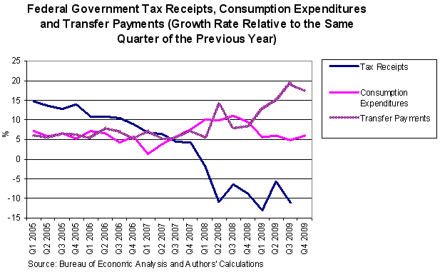
In the aftermath of the Great Recession of 2007, the US federal government budget moved sharply to large deficits. While many attributed this to various fiscal stimulus packages (including bail-outs of the auto industry and Wall Street), the largest portion of the increase in the deficit came from automatic stabilizers and not from discretionary spending. This is easily observable in the graph below which shows the rate of growth of tax revenues (mostly automatic), government consumption expenditures (somewhat discretionary) and transfer payments (again mostly automatic) relative to the same quarter of the previous year:

In 2005 tax revenues were humming, with a growth rate hitting 15% per year—far above GDP growth–hence, reducing non-government sector income—and faster than government spending, which grew just above 5%. Such fiscal tightening (called fiscal drag) often is followed by a downturn—and the downturn that accompanied the GFC was no exception. When it came, the budget deficits increased, mostly automatically. While government consumption expenditures remained relatively stable over the downturn (after a short spike in 2007-2008), the rate of growth of tax revenues dropped sharply from a 5% growth rate to a 10% negative growth rate over just three quarters (from Q 4 of 2007 to Q 2 of 2008), reaching another low of -15% in Q1 of 2009. Tax receipts quite simply fell off a cliff.

Transfer payments grew at an average rate of 10% since 2007, with the higher rate in part due to the rotten economy. Decreasing taxes coupled with increased transfer payments automatically pushed the budget into a larger deficit, notwithstanding the flat consumption expenditures. The automatic stabilizer–and not the bailouts or stimulus—is the main reason why the economy did not go into a freefall as it had in the Great Depression of the 1930s. As the economy slowed, the budget automatically went into a deficit putting a floor on aggregate demand. With countercyclical spending and pro-cyclical taxes, the government’s budget acts as a powerful automatic stabilizer: deficits increase sharply in a downturn.

The expansion before the GFC had been led (mostly) by the 2000s housing boom, during which households borrowed (and spent) on an unprecedented scale. We already visited the three balances that demonstrated the private sector taken as a whole deficit spent for almost a decade in the lead-up to the GFC. In the Clinton boom, about half the deficit spending was by firms; however in the 2000s boom it was entirely the household sector that spent more than its income. Both the Clinton boom and the 2000s boom caused the budget deficit to fall (and to actually move into a large surplus during the Clinton years).

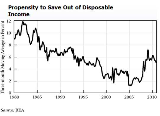
Since the crash, the household sector has retrenched (as it always does in recession), and saving remains high. Slow growth has been the major cause of the rapidly growing budget deficit—and the slow growth, in turn, is due to a high propensity to save by the retrenching household sector. See the next graph (thanks to Dimitri Papadimitriou of the Levy Economics Institute for providing the next two graphs to me):

What we see is a rather remarkable reduction of household saving on trend since the mid-1980s. The cause is beyond the scope of this blog. But the flip-side to that has been the rise of household debt. That trend turned around sharply after the GFC, with households saving like it was 1992 all over again. Given loss of jobs, and stagnant incomes (at best) for most Americans, the notion that the household propensity to spend will sharply reverse course seems unlikely.

As we discussed above, shrinking the government’s deficit will require either that the private sector spend more relative to its income or that the US current account deficit fall sharply. But households are still heavily indebted and indeed more and more homeowners are falling “underwater”—so the likelihood that they will drop saving back down to the 2-3% range we saw in the 2000s seems unlikely. (Note that saving as a percent of disposable income is not exactly the same as the household balance that goes into our three sector balance equation. That is why although this is a small positive saving number, in the sectoral balances equation households actually spent more than their income. See the note at the end of this blog for the wonky stuff.)

Another possibility is a domestic private business sector boom. That, too is unlikely with high unemployment and depressed domestic demand and stagnant sales—investment by firms is not going to grow that much. (I won’t go into it here, but there is a lot of evidence that “investment-led booms” are really residential housing investment booms—housing construction is included in investment numbers–and there is little chance that we will see a housing construction boom in the near future.)

The final possibility is the foreign sector. The next graph shows US imports and exports on current account.

Imports are running around 18% of GDP (rebounding sharply since the GFC) and exports are at 14% of GDP—so exports are up, but imports are climbing a bit faster (this difference is mostly due to oil). While it is true that the US current account balance has become less negative in recent months, much more movement will be required to actually get to positive territory (more than 3% of GDP of adjustment would be required). Note that the last time we actually had a positive current account balance was in the Bush, Sr., recession—two decades ago.

Remember, to reduce the government sector deficit from the current 9% or so of GDP toward balance will require some combination of a private sector movement toward deficit and a current account movement toward surplus amounting to a total of 9% points of GDP. That is huge. The problem is that actually trying to balance the budget through spending cuts or tax increases could reduce economic growth (I think it will actually cause a sharp downturn, but I do not need to make that case). Lower economic growth could conceivably reduce our current account deficit—by making Americans too poor to buy imports, by lowering US wages and prices to make our exports more competitive, and by reducing the value of the dollar. Note that all of those are painful adjustments for Americans. And it might not work, because it requires the US to slow without that affecting the global economy—if it also slows, US exports will not increase.

Now, deficit warriors insist that cutting government will induce faster growth of the private sector. If that were true, it actually makes it easier to reduce the budget deficit—as the private sector’s balance worsens toward deficit. On the other hand, more rapid growth will probably cause deterioration of the current account deficit (our imports will rise; our wages and prices will not fall; and the dollar could gain strength). That in turn must be matched by some combination of private sector and government sector movements toward deficits. The US has a higher propensity to import than do our trading partners—what that means is that if we grow at about the same rate as the rest of the world, our imports grow faster than our exports.

So, to balance the government’s budget we need to grow faster, but faster growth will probably increase our current account deficit so that the three balances identity will imply either that our private sector returns to excessive spending (as it did for the past decade) or that the government’s deficit cannot be reduced. It is something of a Hobson’s choice—with no morality implied—because what appears to be a “free choice” of reducing the budget deficit through faster growth means we actually are accepting bigger household debts and a bigger current account deficit.

That is the problem with analysis and policy recommendations that do not take account of the three balances—they ignore what is implied for the other balances.

Let us summarize the points. First, the three balances must balance to zero. This implies it is impossible to change one of the balances without having a change in at least one other. Second, at the aggregate level, spending (mostly) determines income. A sector can spend more than its income, but that means another spends less. While we can take government spending as more-or-less discretionary, government tax revenue (its equivalent to its income) depends largely on economic performance. Chart 1 above showed that tax receipt growth is highly variable, moving pro-cyclically (growing rapidly in boom and collapsing in slump).

Government can always decide to spend more (yes, it is politically constrained), and it can always decide to raise tax rates (again, given political constraints), but it cannot decide what its tax revenue will be because we apply a tax rate to variables like income and wealth that are outside government control. And that means the budgetary outcome—whether surplus, balanced, or deficit—is not really discretionary.

Turning to our foreign sector, exports are largely outside control of the US (we say they are “exogenous” or “autonomous to US income”). They depend on lots of factors, including growth in the rest of the world, US exchange rates, trade policy, and relative prices and wages (US efforts to increase exports will almost certainly lead to responses abroad). It is true that economic outcomes in the US can influence exports (as discussed, slower US growth can slow global growth)—but impacts of policy on exports are loose.

On the other hand, US imports depend largely on US income (plus exchange rates, relative wages and prices, and trade policy; again, if the US tried to reduce imports this would almost certainly lead to responses by trading partners that are pursuing trade-led growth). Imports are largely pro-cyclical, too. Again, our current account outcome—whether deficit, surplus, or balanced—is also largely nondiscretionary.

What is discretionary? Domestic spending—by households, firms, and government—is largely discretionary. And spending largely determines our income. Sectoral balances, however, should be taken as mostly nondiscretionary because they depend in very complex ways on the discretionary variables plus the nondiscretionary variables and on the constraints imposed by the macro identity. It makes most sense to promote spending that will utilize domestic resources close to capacity, and then let sectoral balances fall where they may. As we will argue in coming months, the best domestic policy is to pursue full employment and price stability—not to target arbitrary government deficit or debt limits, which are mostly nondiscretionary, anyway.

Note 1: The main differences between the personal saving rate and the household net saving as a % of GDP are the following (thanks to Scott Fullwiler):

1. Household net saving is as a % of GDP, whereas personal saving rate is as a % of disposable income
2. Household net saving subtracts all household spending, including consumption and residential investment, whereas personal saving only subtracts consumption spending

A few additional smaller differences for the really wonky:

1. Household net saving adds an allowance for household capital consumption (i.e., depreciation), personal saving doesn’t,
2. Household net saving imputes insurance and pension reserves to households from govt sector, personal saving doesn’t, and
3. Household net saving includes wage accruals less disbursements from businesses to households, personal saving doesn’t.

Note 2: Thanks to the MMT gang. You know who you are.

There were a large number of relevant comments and questions. I have done some cut and paste here and will deal with them in order.

Question: Is there any material difference between the sectoral balances in a currency and the sectoral balances issued in the national accounts for GDP purposes?

Answer: Here is my understanding: for the US there would be no (significant) difference as we use dollars in our stocks and our flows. Even if we buy foreign made output, we provide dollars that are exchanged for foreign currency. In other countries there could well be a significant portion of the economy that is denominated in a foreign (dollar) currency. Much of that could go unrecorded, of course. In that case the official accounts would be in domestic currency but if it were feasible we could also keep some accounts in dollars. All the macroidentities for this country would still apply for transactions that take place in dollars.

Q: Several comments were made about this statement: “No matter how much others might want to accumulate financial wealth, they will not be able to do so unless someone is willing to deficit spend.”

1. So do you consider inventory run up to be in the category of ‘willing’?
2. I’m thinking optimist makes perishable goods that in the end nobody wants to buy having somehow managed to persuade a bank to create the necessary money (possibly by having large valuable real thing to offer as collateral).
3. I also find it very confusing. A desire to accumulate wealth is very easy to realize – do not spend your income. Whenever anybody gets a paycheck technically the whole amount is saved. So saving or accumulation is realized by definition while spending requires action.

A: If a firm is producing “widgets” it does so to “realize” them in the form of money things—it wants to sell them to get a credit to its bank account If it cannot sell them, they are added to inventory and count in the GDP accounts (technically NIPA) as investment. There will be an offsetting flow which is saving. Within the private sector, the increase to investment equals the increase to saving—this activity has no impact on the overall private sector’s balance. But let us imagine that foreigners order those widgets; in that case, the firm gets to sell them (receiving a credit to its bank account); there will be no increase to domestic investment. Instead, exports have increased—there is a positive entry to the current account balance. Ignoring all other entries, the US domestic private sector gets a surplus on its balance (saving) while the foreign sector “deficit spends”.

I know this will not answer all possible questions that follow on from this. After we look at the “circuit approach” later in the MMP we will see how the firm financed its production of widgets and what the implication is for the firm if it fails to “realize” them in the form of sales for money things. You can think of the “saving” of the household sector as the counterpart to the undesired inventory accumulation by the widget manufacturer. The manufacture of the widget produces household income that can be consumed or saved; of course the firms hope workers never save—because that means lost potential sales. If households do save, widgets go to inventory as investment. The firm can then be in trouble—not able to cover its costs. But foreigners or the government can step in to fill the demand gap.

Q: I wonder about “a) Individual spending is mostly determined by income.” Is this important/necessary/useful for you exposition?

A: Of course, it is true that wealthier people can fairly easily spend even if their flow of income is zero—they can sell off assets or borrow against them. But for many households, it is “mostly” true that income determines spending. And it is common sense to most people. My bigger point, however, is that at the aggregate level we need to think about reversing the causation. My household’s income is mostly determined by my employer’s decision to spend on my wages and salaries. So household consumption really depends to a great extent on its income (so consumption is called “induced spending) but its income in turn comes from somewhere—largely spending by firms and governments on wages, profits, and interest. At that spending by firms is undertaken on the expectation of sales (expenditures by households or other firms). We then also have government and investment and exports that are at least to some extent “autonomous” to income (don’t depend on today’s income). Yes these are important issues both for explanation and for projections of economic performance. There is also a logical angle: a society can decide to spend more but it cannot decide to have more income (unless it spends more). Spending is thus logically prior.

Q: When somebody hands you a five dollar bill, you can’t spend (create an outflow) out of that instantaneous inflow. You can only spend out of your stock — whether it’s a Swiss bank account or the buck and a quarter you have in your pocket. Flows are strings of instantaneous events; stocks have existence and duration. You can only spend out of wealth, not out of income. Obvious, but a point of confusion out there in the world.

A: When my boss pays me my $5 wages, that is indeed an income flow—ie: $5 per hour, per week, per month, or per year. Flows occur over time (even if the time is short). I can accumulate my income (wages) flow in the form of green paper dollar notes—the flows accumulate to a stock of dollar bills. (Stocks are measured at a point in time. Now!, for example.) If instead I spend the wages as I receive them, that is a consumption flow financed out of wages flow. But if I save all my wages as accumulated stacks of dollar bills for a period of a year, and then at the end of the year I choose to run down my wealth by splurging on a new BMW, then I am dissaving (reducing stock of wealth) to finance consumption.

Note that if I accumulated BMWs as my wealth (rather than dollar notes) then I would first have to sell the BMWs before I could finance consumption. That is of course the advantage of accumulating “cash”—I don’t have to sell it before spending. So my exposition was not confused. You could say that it is rather arbitrary whether to count hoarding of $5 notes as a saving flow into my stock of wealth, that I then run down to finance consumption versus spending the $5 income flow to finance consumption. That is to say, as we collapse the time period toward an “instant” then the distinction between flows and stocks disappears. That seems to be what you are saying. An instantaneous flow reduces to a stock as time approaches zero. And that of course is correct, too.

Note that income can be received as a flow of claims (rather than green paper). I work all month long, accumulating wage claims on my employer. (Legally enforceable in court.) Then I finally get my paycheck and deposit it in my bank account. Now I spend down my deposit until my next paycheck. If we want to be technically wonky we would say you are receiving an income flow every day of the month that finances a consumption flow every day of the month. But as you say, the “payment” of the wage actually takes place on a single day as a credit to your bank account (increasing your stock of wealth). (Technically, the claim on your employer is converted to a bank deposit—usually a debit to your employer’s account and a credit to yours.) You could not “really” spend your wages (claims on your employer) until you got your paycheck—except by borrowing against the claims.

Q: My understanding of domestic government budget surpluses is that they merely destroy the dollars that earlier spending created. Isn’t it meaningless to suggest that a sovereign government “saves” its own fiat currency?

A: In practical terms, yes. In the US during the Clinton boom there was a projection that all outstanding US Treasury debt would be retired. This led to a mad rush at the Fed to figure out how the federal government could continue to run surpluses if there were no government IOUs out there to “destroy”. If we ever did get to that point, the only way the private sector could continue to run deficits against the government would be to surrender assets (not government IOUs) in payment. You’d have to turn over your car, house, bank account, and children to the government to pay taxes!! That is the logical result of a government surplus carried to infinity—government would accumulate infinite claims on you. And yes you are correct that sovereign government does not—cannot—“save” its own currency!

Q: “It is impossible for every individual in the private domestic sector to net save at the same time if that sector’s aggregate balance is zero” Sure, but the logic is not the one you and this post claim. It is savers who force deficit spending and not the other way. This is the reason why.

A: Takes two to tango, of course. I think I made that clear. But carrying on from above, at the aggregate level (at least) it makes more sense to say that spending “causes” income which in turn “causes” saving. Here is why. If I am credit worthy I can always decide to spend more (the bank takes my IOU, gives me its IOU, and I deficit spend). I cannot (easily) decide to have more income. I need income to save more. Still, it takes two to tango. Yes, if I have income I can decide to consume less and save more. That will have an implication on someone else’s income flow (since I am not buying her widgets). And that means undesired deficit spending (and perhaps inventory accumulation—as above).

Q: Could you provide an algebraic description of MMT and its prescriptions as part of the MMP?

A: I did.

Domestic Private Balance + Domestic Government Balance + Foreign Balance = 0

That is pretty much all the math(s) you need to become a good macroeconomist! If you understand that, you are way ahead of most Nobel winners. (More seriously, where math helps, we will use it.)

In Blog #2 we introduced the basics of macro accounting, and in Blog #3 we took a break from accounting to take a look at the rise and fall of the Goldilocks economy in the US. Thus, we applied our sectoral balance identity to the case of the US. In today’s blog we will go a bit deeper into the accounting, looking at the relation between flows (deficits) and stocks (debts). To avoid making mistakes we need to make sure that we have “consistency” between our flows and our stocks. We want to make sure that all spending and saving comes from somewhere and goes somewhere. And we must make sure that one sector’s surplus is offset by a deficit in another sector. This is a lot like keeping track of the scores in a baseball game, and in fact most financial “scores” really are electronic entries in the modern world.

We will also try to say something about causation. It is not sufficient to say that at the aggregate level, the private balance plus the government balance plus the foreign balance equals zero. We would like to be able to understand why the private sector balance was negative during the Clinton Goldilocks years while the government balance was positive—how did we get to that point, and what sorts of processes did it induce. Obviously that is necessary before we can really analyse the situation and formulate policy. Unlike the macro accounting identity (which must be true), it is not possible to say with certainty what causes a particular sector’s balance. It is quite easy to say that if the government runs a surplus and if the foreign balance is positive (foreign sector spends less than its income) then the domestic private sector must by accounting identity be negative (running a deficit). It all must sum to zero.

Explaining why the private sector had a deficit during the Goldilocks years is harder; it is even harder to project if and for how long that deficit would continue. I already made clear in Blog 3 that I got the timing wrong—private sector deficits continued for about 4 years longer than I expected. Projections are darned hard to get right—if they were easy, MMTers would all make lots of money placing bets on outcomes. Another way of stating this is to say that a good understanding of MMT does not give one any monopoly on explanations of causation. We must not be overly confident. As the late and great Wynne Godley used to put it, he did not make forecasts, rather, he made contingent projections.

For example, carrying on with the work of Godley, the Levy Economics Institute (www.levy.org) makes such projections. Typically it begins with CBO (Congressional Budget Office) projections of the path of government deficits and of economic growth over the next few years. CBO projections are largely determined by current law (ie: laws determining government spending and taxing, as well as mandates over deficit reduction). However, the CBO’s projections are not stock-flow consistent and do not adopt the three sector balances approach (this used to drive Godley crazy). In other words, they are incoherent. But given projections over the government balance and GDP growth as well as empirical estimates of various economic parameters (propensity to consume and import, for example), one can produce a stock-flow consistent model that produces the implied sectoral balances as well as path of debt. The Levy Institute often finds that economic growth rates (for example) plus government deficit projections used in CBO forecasts imply highly implausible balances in the other two sectors (domestic private and foreign) as well as private debt ratios. To do that kind of analysis, you must go beyond the simple accounting identities.

Deficits -> savings and debts -> wealth. We have established in our previous blogs that the deficits of one sector must equal the surpluses of (at least) one of the other sectors. We have also established that the debts of one sector must equal the financial wealth of (at least) one of the other sectors. So far, this all follows from the principles of macro accounting. However, the economist wishes to say more than this, for like all scientists, economists are interested in causation. Economics is a social science, that is, the science of extraordinarily complex social systems in which causation is never simple because economic phenomena are subject to interdependence, hysteresis, cumulative causation, and so on. Still, we can say something about causal relationships among the flows and stocks that we have been discussing in the previous blogs. Some readers will note that the causal connections adopted here follow from Keynesian theory.

a) Individual spending is mostly determined by income. Our starting point will be the private sector decision to spend. For the individual, it seems plausible to argue that income largely determines spending because one with no income is certainly going to be severely constrained when deciding to purchase goods and services. However, on reflection it is apparent that even at the individual level, the link between income and spending is loose—one can spend less than one’s income, accumulating net financial assets, or one can spend more than one’s income by issuing financial liabilities and thereby becoming indebted. Still, at the level of the individual household or firm, the direction of causation largely runs from income to spending even if the correspondence between the two flows is not perfect. There is little reason to believe that one’s own spending significantly determines one’s own income.

b) Deficits create financial wealth. We can also say something about the direction of causation regarding accumulation of financial wealth at the level of the individual. If a household or firm decides to spend more than its income (running a budget deficit), it can issue liabilities to finance purchases. These liabilities will be accumulated as net financial wealth by another household, firm, or government that is saving (running a budget surplus). Of course, for this net financial wealth accumulation to take place, we must have one household or firm willing to deficit spend, and another household, firm, or government willing to accumulate wealth in the form of the liabilities of that deficit spender. We can say that “it takes two to tango”. However, it is the decision to deficit spend that is the initiating cause of the creation of net financial wealth. No matter how much others might want to accumulate financial wealth, they will not be able to do so unless someone is willing to deficit spend.

Still, it is true that the household or firm will not be able to deficit spend unless it can sell accumulated assets or find someone willing to hold its liabilities. We can suppose there is a propensity (or desire) to accumulate net financial wealth. This does not mean that every individual firm or household will be able to issue debt so that it can deficit spend, but it does ensure that many firms and households will find willing holders of their debt. And in the case of a sovereign government, there is a special power—the ability to tax–that virtually guarantees that households and firms will want to accumulate the government’s debt. (That is a topic we pursue later.) We conclude that while causation is complex, and while “it takes two to tango”, causation tends to run from individual deficit spending to accumulation of financial wealth, and from debt to financial wealth. Since accumulation of a stock of financial wealth results from a budget surplus, that is, from a flow of saving, we can also conclude that causation tends to run from deficit spending to saving.

c) Aggregate spending creates aggregate income. At the aggregate level, taking the economy as a whole, causation is more clear-cut. A society cannot decide to have more income, but it can decide to spend more. Further, all spending must be received by someone, somewhere, as income. Finally, as discussed earlier, spending is not necessarily constrained by income because it is possible for households, firms, or government to spend more than income. Indeed, as we discussed, any of the three main sectors can run a deficit with at least one of the others running a surplus. However, it is not possible for spending at the aggregate level to be different from aggregate income since the sum of the sectoral balances must be zero. For all of these reasons, we must reverse causation between spending and income when we turn to the aggregate: while at the individual level, income causes spending, at the aggregate level, spending causes income.

d) Deficits in one sector create the surpluses of another. Earlier we showed that the deficits of one sector are by identity equal to the sum of the surplus balances of the other sector(s). If we divide the economy into three sectors (domestic private sector, domestic government sector, and foreign sector), then if one sector runs a deficit at least one other must run a surplus. Just as in the case of our analysis of individual balances, it “takes two to tango” in the sense that one sector cannot run a deficit if no other sector will run a surplus. Equivalently, we can say that one sector cannot issue debt if no other sector is willing to accumulate the debt instruments.

Of course, much of the debt issued within a sector will be held by others in the same sector. For example, if we look at the finances of the private domestic sector we will find that most business debt is held by domestic firms and households. In the terminology we introduced earlier, this is “inside debt” of those firms and households that run budget deficits, held as “inside wealth” by those households and firms that run budget surpluses. However, if the domestic private sector taken as a whole spends more than its income, it must issue “outside debt” held as “outside wealth” by at least one of the other two sectors (domestic government sector and foreign sector). Because the initiating cause of a budget deficit is a desire to spend more than income, the causation mostly goes from deficits to surpluses and from debt to net financial wealth. While we recognize that no sector can run a deficit unless another wants to run a surplus, this is not usually a problem because there is a propensity to net save financial assets. That is to say, there is a desire to accumulate financial wealth—which by definition is somebody’s liability.

Conclusion. Before moving on it is necessary to emphasize that everything in this blog (as well as Blog #2) applies to the macro accounting of any country. While examples used the dollar, all of the results apply no matter what currency is used. Our fundamental macro balance equation,

Domestic Private Balance + Domestic Government Balance + Foreign Balance = 0

will strictly apply to the accounting of balances of any currency. Within a country there can also be flows (accumulating to stocks) in a foreign currency, and there will be a macro balance equation in that currency, too.

Note that nothing changes if we expand our model to include a number of different countries, each of which issues its own currency. There will be a macro balance equation for each of these countries and for each of the currencies. Individual firms or households (or, for that matter, governments) can accumulate net financial assets denominated in several different currencies; vice versa, individual firms or households (or governments) can issue net debt denominated in several different currencies. It can even become more complicated, with an individual running a deficit in one currency and a surplus in another (issuing debt in one currency and accumulating wealth in another). Still, for every country and for every currency there will be a macro balance equation.

OK that is enough for this week. Can I remind commentators and questioners that this is a Primer. We will collect questions and comments until Wednesday and then post a response. We appreciate comments and questions directly related to this blog. We really do not want comments from those who have already examined and rejected MMT.

Thank you for comments and questions. Let me divide the responses into several different issues.

1. “Sustainability Conditions” for Government Deficits

I said: “If you want to take a guess at what our “mirror image” in the graph above will look like after economic recovery, I would guess that we will return close to our long-run average: a private sector surplus of 2% of GDP, a current account deficit of 3% of GDP and a government deficit of 5% of GDP. In our simple equation it will look like this:

Private Balance (+2) + Government Balance (-5) + Foreign Balance (+3) = 0.

And so we are back to the concept of zero!”

Now I want to be clear, I said nothing to imply these particular sectoral balances would continue on through infinity to the sweet hereafter. What I gave was a contingent statement (what the balances would look like AFTER recovery and if we return to LONG-RUN AVERAGES—that is to say, average stances over the past 30 years or so, taking into account trends—essentially just eye-balling the 3 sectors graph provided in the blog). I have made no projection that we actually WILL recover, and it is certainly possible that even after recovery our private sector balance will remain in high surplus. Let us say it remains at 6% (which would be higher than average but consistent with an attempt to delever debt—that is, to keep consumption low in order to pay down debt). In that case, and again assuming the foreign balance remains a positive 3% (that is, our current account deficit is 3%) then the government will remain in deficit of 9% (more or less where it is now). I will not place probabilities on these two outcomes—I think the original statement is more likely—because my main point is simply that taking balances of each of the 3 sectors, the overall balance must be 0.

For those who would like to balance the government budget, the burden is on them to tell me what the implied outcome for the private and foreign sectors will be. If we are not going to return to the disastrous “Goldilocks” outcome with the private sector running deficits, then a huge adjustment will be necessary in the foreign balance in order to have a balanced government budget with a private sector surplus. Virtually none of the deficit hawks consider this. But, again, I would like to hear their explanation for how we will get the current account into surplus.

On to the sustainability conditions. It has become trendy among economist wonks to look at government budget stances to determine whether they could continue forever. Many objections could be raised to such purely mental exercises. An obvious one is that no government has ever lasted forever—and so any such exercise is a waste of time. Ok that one is not something we want to contemplate. Economist Herb Stein quipped that unsustainable processes will not be sustained. Something will change. That gets us somewhat closer to the problem with such approaches. And finally, if we are dealing with sovereign budget deficits we must first understand WHAT is not sustainable, and what is. That requires that we need to do sensible exercises. The one that the deficit hysterians propose is not sensible.

Let us first look at a somewhat simpler unsustainable process. Suppose that some guy—we’ll use the name Ramanan—decides to replicate the “Supersize me” experiment (based on the 2004 documentary by Morgan Spurlock). His caloric intake is 5000 calories a day, and he burns 2000 daily. The excess 3000 calories lets him gain one pound of body weight each day. If he weighed 200 pounds on January 1, by the end of the year he weighs 565 pounds. After 100 years he’s up to 36,700 pounds—a bit on the pudgy side. But we don’t stop there. After 100,000 years he weighs 36,700,000 pounds, and after a few million years, he’s heavy enough to affect the earth’s spin on its axis and its revolutions about the sun. But, according to our policy wonks, that still is not a long enough period—we’ve got to carry this out to infinity, at which point, Ramanan is infinite sized, like the universe, and if he is growing faster than the expansion of the universe, the entire rest of the universe will eventually be infinitesimally smaller than Ramanan. I guess he’s become the black hole of the universe (but I’m no physicist or biologist). So, yes this is unsustainable. Aren’t we all clever?

But would the process actually work that way? Of course not. First, Ramanan is not going to live an infinite number of years; second, he’s either going to blow up (literally) or go on a diet; and third, and most important, his body is going to adjust. As his body mass increases, he will burn more than 2000 calories a day—perhaps he’ll get up to a 5000 calorie a day burn-rate—and his body will use the food in a less efficient manner. So he will stop gaining weight long before he becomes the universe’s black hole. Herb Stein was right.

Our little mental exercise was fundamentally flawed. It assumed a fixed caloric input (flow) and a fixed caloric burn-rate (consumption flow) with the difference between the two accumulating as a stock (weight gain) at a fixed rate (essentially, “savings”). No adjustments to behavior or metabolism are allowed. And then the whole absurd set-up is carried to the ultimate absurdity by the use of infinite horizon projections. Anything carried to a logical absurdity is unsustainable. As you will see, this is the rigged game used by deficit warriors to “prove” the US Federal budget deficit is unsustainable.

The trick used by deficit warriors is similar but with the inputs and outputs reversed. Rather than caloric inputs, we have GDP growth as the input; rather than burning calories, we pay interest; and rather than weight gain as the output we have budget deficits accumulating to government debt outstanding. To rig the little model to ensure it is not sustainable, we have the interest rate higher than the growth rate—just as we had Ramanan’s caloric input at 5000 calories and his burn rate at only 2000—and this will ensure that the debt ratio grows (just as we ensured that Ramanan’s waistline grew without limit). Let us see how this works.

We will start with a simple example similar to the one used in our blog and response last week. Let us have two sectors, government and private. Our government follows the Goldilocks model, spending less than its income (tax revenue); the private sector by identity runs a deficit (spends more than its income). We know this means the private sector is running up debt, held by the government as its asset (surpluses are realized in the form of private sector IOUs). The private sector must service the debt by paying interest; that of course adds to its deficit (interest is additional spending it must make out of its income). In comparison to our Supersizing Ramanan, the sustainability conditions will be determined by the interest rate paid, the growth rate of income (or GDP), and the deficit of the private sector.

Jamie Galbraith laid out the typical model used to evaluate sustainability of deficit spending as follows:

The key formula is:

Δd = –s + d * [(r – g)/(1 + g)]

Here, d is the starting ratio of debt to GDP, s is the “primary surplus” or budget surplus after deducting net interest payments (as shares of GDP), r is the real interest rate, and g is the real rate of GDP growth. (http://www.levyinstitute.org/publications/?docid=1379)

Now, this is wonky but the key idea is that (given a relation between the primary surplus and starting debt–both as ratios to GDP) so long as the interest rate (r) is above the growth rate (g) the debt ratio is going to grow. (Jamie has put these key terms in “real”—that is inflation adjusted—terms but that really does not matter; we can keep it all in nominal terms since “deflation” by the inflation rate merely reduces all terms by the inflation rate). Note that the starting debt ratio (d) as well as the primary surplus (what the private sector’s budget would be if it did not have to pay interest) also play a role. (Galbraith proves that the starting debt ratio does not matter much—just as Ramanan’s initial weight will not matter since in any case he will grow to an infinite size.) But we do not need to get too hung up in math to see that all things equal if the interest rate is above the growth rate, we get a rising debt ratio. If we carry this through eternity, that ratio gets big. Really big. Ok that sounds bad. And it is. Remember, that is a big part of the reason that the GFC hit—overindebted private sector. The GFC is the equivalent to an explosion of Ramanan that would prevent him from growing to an infinite size. (A debt diet would have been far preferable, but Greenspan and Bernanke opposed “interfering” with Wall Street lender fraud.)

Now let us change all this around. Let us say that the government runs a continuous budget deficit while the private sector runs a surplus. We can obtain the same equation. It appears that a continuous government budget deficit implies a continuously rising debt to GDP ratio and surely that is unsustainable. (See the appendix below for more complex math.)

But wait a minute. Is such a mental exercise sensible? We already saw that our supersizing Ramanan is going to adjust: he will diet, explode, increase his metabolism, and reduce the efficiency of his absorption of calories. If he does not explode, he will reach some “equilibrium” in which his intake of calories will equal his burn-rate so that his waistline will stop growing. What about our supersizing government? Here are the possible consequences of a persistent deficit that implies rising interest payments and debt ratios:

1. Inflation: this tends to increase tax revenues so that they grow faster than government spending, thus lowering deficits. (Many, including Galbraith, would point to the tendency to generate “negative” interest rates.) In other words the growth rate will rise above the interest rate, and reverse the dynamics so that the debt ratio stops growing. (That is equivalent to an increase of Ramanan’s caloric burn rate—so he stops growing.)
2. Austerity: government can try to adjust its fiscal stance (increasing taxes and reducing spending to lower its defict). Of course, it takes “two to tango”—raising tax rates might not change the government’s balance. It could lower growth rates, and thereby actually increase the rate of growth of the debt ratio.
3. The private sector will adjust its flows (spending and saving) in response to the government’s stance. If government continually spends more than its income, it will be adding net wealth to the private sector; and its interest payments will add to private sector income. It is not plausible to believe that as the government’s debt ratio goes toward infinity (which means that the private sector’s net wealth ratio goes to infinity) there is no induced spending in the private sector. That is usually called the “wealth effect”. In other words, government debt is private wealth and as private wealth grows without limit this will eventually cause spending to rise relative to private sector income—reducing government deficits. In addition, private sector income includes government interest payments, so rising government interest payments on its debt could induce consumption. When all is said and done, the private sector will not be happy consuming less than its income flow—given its rising wealth—and will adjust its saving behavior. If the private sector tries to reduce its surpluses, this can be done only by reducing the government sector’s deficits. It takes two to tango and the likely result is that tax revenues and consumption will rise, the government’s deficit will fall, and the private sector’s surplus will fall.
4. Government deficit spending and interest payments could increase the growth rate; it can be pushed above the interest rate. This changes the dynamics and can stop the growth of the debt ratio.
5. The interest rate is a policy variable (as will be discussed in subsequent weeks). Ignoring all the dynamics discussed in the previous points, to avoid an exploding debt ratio, all the government needs to do is to lower the interest rate below the economic growth rate. End of story, sustainability achieved.

Finally, and this is the most contentious point. Suppose none of the dynamics just discussed come into play, so the government’s debt ratio rises on trend. Will a sovereign government be forced to miss an interest payment—no matter how big that becomes? The answer is a simple “no”. It will take weeks of explication of MMT to explain why. But let us put this in the simple terms that Chairman Bernanke used to explain all the Fed spending to bail-out Wall Street: government spends using keystrokes, or, electronic entries on balance sheets. There is no technical or operational limit to its ability to do that. So long as there are keyboard keys to stroke, government can stroke them to produce interest payments credited to balance sheets.

And that finally gets us to the difference between perpetual private sector deficit spending versus perpetual government sector deficits: the first really is unsustainable while the second is not. Now, I want to be clear. We have argued that persistent government budget deficits that increase government debt ratios and thus private wealth ratios will lead to behavioral changes. They could lead to inflation. They could lead to policy changes. Hence, they are not likely to last “forever”. So when I say they are “sustainable” I merely mean in the sense that sovereign government can continue to make all payments as they come due—including interest payments—no matter how big those payments become. It might choose not to make those payments. And the mere act of making those payments will likely cause changes in growth rates and budget deficits and growth of debt rations.

2. “Sustainability” of Current Account ratios:

In the quote at the top of this response there was also a contingent statement about US current account deficits. To be more clear (and thus to respond to comments), the current account includes the balance of trade (and, more broadly, the balance between exports and imports) plus some other items including “factor payments” (interest and profits paid and received). For the US, we obviously run a trade deficit (and exports are less than imports), but the factor payments are in our favor (we receive more in profits and interest from abroad than we pay to foreign creditors and owners). In any event, our negative current account balance is offset by a positive capital account balance. To put it simply—there is a “flow” of dollars abroad due to the current account deficit that is matched by the “flow” of dollars back to the US due to our capital account surplus. This is often (misleadingly) presented as US “borrowing” of dollars to “pay for” our trade deficit. We could just as well put it this way: the US imports more than it exports because the rest of the world wants to accumulate savings in dollar-denominated assets. I do not want to go into that in detail since it is the subject of later blogs.

But here’s the question. Is a continuous current account deficit possible? A simple answer is yes, so long as “two want to tango”: if the rest of the world wants dollar assets and Americans want rest of world exports (imported to the US), this will continue. But, hold it, say the worriers. As the rest of the world accumulates dollar claims on the US, they also receive interest payments. That is a factor payment that increases our current account deficit. You can see the relation to the point above about government deficits and interest payments. The world will be flooded with dollars twice over: once from our excessive propensity to import and once from our interest payments on debt.

But here is the interesting point: even though the US is the “biggest debtor on earth”, those factor payments flow in our favor. We pay extremely low interest rates and profit rates to foreigners, and earn much higher interest rates and profits on our holdings of foreign investments and debt. Why is that? Because the US is the safest investment on earth. Anytime there is a financial crisis anywhere in the world, where do international investors run? To the US dollar. Ironically, that happens even when the crisis begins in the US! Why? The US has a sovereign government with a sovereign currency. Its interest rate is set by the Fed, which can always set the rate below the US growth rate (and, indeed, as Galbraith points out, the inflation-adjusted interest rate is often below the “real” growth rate). In spite of the deficit hysteria whipped up by hedge fund billionaire Pete Peterson, no investor in her right mind believes there is any default risk on US Treasury debt. So when global fears rise, investors run to the dollar. This could change, but not in your lifetime.

In short, I make no projection about continued US current account deficits but I believe they will continue far longer than anyone imagines. They are sustainable. They will be sustained until the rest of the world decides not to accumulate more dollars and Americans decide they really do not want the cheap junk and environment-destroying oil produced by the rest of the world. When that will happen, I do not know. It is nothing to lose sleep over. Yes we can calculate “sustainability conditions” but it would just be an exercise in mental masturbation. We’ve already done enough of that. I suppose it is titillating but ultimately unsatisfying.

3. Briefly there were several other points raised.

There were some about maldistribution of income as a contributing cause of the private sector deficit. Agreed. There were some questions about stocks and relations to flows. Some of that is treated above but much more will come in the next series of blogs. There were points made about need to regulate Wall Street. Yes! There were questions about QE and the difference between helicopter drops and fiscal policy. Put it this way: Treasury SPENDS money things into existence, the Fed LENDS money things into existence. The first adds income and net wealth, the second only transforms balance sheets. This will be explained in more detail later.

Appendix:

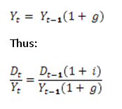
Government debt outstanding (D) follows the following law of motion:

That is, every year, assuming the debt never matures, the outstanding debt increases by the size of the deficit. The deficit is the difference between government spending (G), taxes (T) plus interest payments on outstanding debt (iD)

Let us assume to simplify that G = T so: therefore

The gross domestic product (Y) grows at a rate g and so follows the following law of motion:

Let us find the limit of this ratio:

Following the same logic for Y we get (noting d the debt to gdp ratio)

It is pretty clear that if i > g then the ratio tends toward infinity when n tends toward infinity; and toward zero otherwise. If g = i then dt = d0 for all t.

The complication of the deficit to GDP ratio at 5% would mean:

Without going too far into the implications we have:

Therefore by doing a recursive calculation we get:

As n tends toward infinity dt also does. Note that a given deficit to gdp ratio means that deficit has to explode as gdp increases.

Thanks: to James Galbraith and Eric Tymoigne.

In the previous blog, we did some heavy lifting. Unless you are an economics or accounting nerd, you found it quite boring. This week we will take a little break from pure accounting, and apply what we’ve learned to a real world example. By now, long-time readers are quite familiar with the NEP’s approach to the GFC (global financial crisis). Let us revisit the Clintonian Goldilocks economy to find the seeds of the GFC, using our sectoral balance approach.

To be clear, what follows uses our sectoral balances identity plus some real world data to provide an interpretation of the causes of the crash. As always, interpretations are subject to disagreement. The identity as well as the data are not. (You can of course always begin analysis with other identities and other data.) Next week we return to a bit more accounting.

Back in 2002 I wrote a paper announcing that forces were aligned to produce the perfect fiscal storm. (I note that in recent days a few analysts—including Nouriel Roubini—have picked up that terminology.) What I was talking about was a budget crisis at the state and local government levels. I had recognized that the economy of the time was in a bubble, driven by what I perceived to be unsustainable deficit spending by the private sector—which had been spending more than its income since 1996. As we now know, I called it too soon—the private sector continued to spend more than its income until 2006. The economy then crashed—a casualty of the excesses. What I had not understood a decade ago was just how depraved Wall Street had become. It kept the debt bubble going through all sorts of lender fraud; we are now living with the aftermath.

Still, it is worthwhile to return to the so-called “Goldilocks” period (mid to late 1990s, said to be “just right”, with growth sufficiently strong to keep unemployment low, but not so swift that it caused inflation) to see why economists and policymakers still get it wrong. As I noted in that earlier paper,

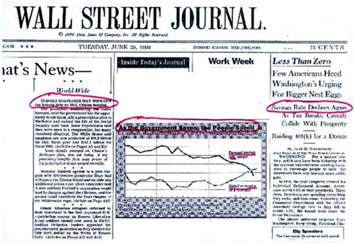
It is ironic that on June 29, 1999 the Wall Street Journal ran two long articles, one boasting that government surpluses would wipe out the national debt and add to national saving—and the other scratching its head wondering why private saving had gone negative. The caption to a graph showing personal saving and government deficits/surpluses proclaimed “As the government saves, people spend”. (The Wall Street Journal front page is reproduced below.) Almost no one at the time (or since!) recognized the necessary relation between these two that is implied by aggregate balance sheets. Since the economic slowdown that began at the end of 2000, the government balance sheet has reversed toward a deficit that reached 3.5% of GDP last quarter, while the private sector’s financial balance improved to a deficit of 1% of GDP. So long as the balance of payments deficit remains in the four-to-five percent of GDP range, a private sector surplus cannot be achieved until the federal budget’s deficit rises beyond 5% of GDP (as we’ll see in a moment, state and local government will continue to run aggregate surpluses, increasing the size of the necessary federal deficit). [I]n recession the private sector normally runs a surplus of at least 3% of GDP; given our trade deficit, this implies the federal budget deficit will rise to 7% or more if a deep recession is in store. At that point, the Wall Street Journal will no doubt chastise: “As the people save, the government spends”, calling for a tighter fiscal stance to increase national saving!

Turning to the international sphere, it should be noted that US Goldilocks growth was not unique in its character. [P]ublic sector balances in most of the OECD nations tightened considerably in the past decade–at least in part due to attempts to tighten budgets in line with the Washington Consensus (and for Euroland, in line with the dictates of Maastricht criteria). (Japan, of course, stands out as the glaring exception—it ran large budget surpluses at the end of the 1980s before collapsing into a prolonged recession that wiped out government revenue and resulted in a government deficit of nearly 9% of GDP.) Tighter public balances implied deterioration of private sector balances. Except for the case of nations that could run trade surpluses, the tighter fiscal stances around the world necessarily implied more fragile private sector balances. Indeed, Canada, the UK and Australia all achieved private sector deficits at some point near the beginning of the new millennium. (Source: L. Randall Wray, “The Perfect Fiscal Storm” 2002, available at http://www.epicoalition.org/docs/perfect_fiscal_storm.htm)

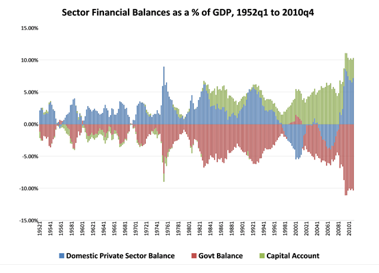
Let us revisit “Goldilocks” and see what lessons we can learn from “her” that help us to understand the Global Financial Collapse that began in 2007. As we now know, my short-term projections predicting the demise of Goldilocks into a recession were not too bad, but the medium-term projections were off. The Bush deficit did grow to 5% of GDP, helping the economy to recover. But then the private sector moved right back to huge deficits as lender fraud fuelled a real estate boom as well as a consumption boom (financed by home equity loans). See the chart below (thanks to Scott Fullwiler). Note that we have divided each sectoral balance by GDP (since we are dividing each balance by the same number—GDP—this does not change the relationships; it only “scales” the balances). This is a convenient scaling that we will use often in the MMP. Since most macroeconomic data tends to grow over time, dividing by GDP makes it easier to plot (and rather than dealing with trillions of dollars—so many zeroes!—we express everything as a percent of total spending).

This chart shows the “mirror image”: a government deficit from 1980 through to the Goldilocks years is the mirror image of the domestic private sector’s surplus plus our current account deficit (shown as a positive number because it reflects a positive capital account balance—the rest of the world runs a positive financial balance against us). (Note: the chart confirms what we learned from Blog #2: the sum of deficits and surpluses across the three sectors must equal zero.) During the Clinton years as the government budget moved to surplus, it was the private sector’s deficit that was the mirror image to the budget surplus plus the current account deficit.

This mirror image is what the Wall Street Journal had failed to recognize—and what almost no one except those following the Modern Money approach as well as the Levy Economic Institute’s researchers who used Wynne Godley’s sectoral balance approach understand. After the financial collapse, the domestic private sector moved sharply to a large surplus (which is what it normally does in recession), the current account deficit fell (as consumers bought fewer imports), and the budget deficit grew mostly because tax revenue collapsed as domestic sales and employment fell.

Unfortunately, just as policymakers learned the wrong lessons from the Clinton administration budget surpluses—thinking that the federal budget surpluses were great while they actually were just the flip side to the private sector’s deficit spending—they are now learning the wrong lessons from the global crash after 2007. They’ve managed to convince themselves that it is all caused by government sector profligacy. This, in turn has led to calls for spending cuts (and, more rarely, tax increases) to reduce budget deficits in many countries around the world (notably, in the US and UK).

The reality is different: Wall Street’s excesses led to too much private sector debt that crashed the economy and reduced government tax revenues. This caused a tremendous increase of federal government deficits. {As a sovereign currency-issuer, the federal government faces no solvency constraints (readers will have to take that claim at face value for now—it is the topic for upcoming MMP blogs).} However, the downturn hurt state and local government revenue. Hence, they responded by cutting spending, laying-off workers, and searching for revenue.

The fiscal storm that killed state budgets is the same fiscal storm that created the federal budget deficits shown in the chart above. An economy cannot lose about 8% of GDP (due to spending cuts by households, firms and local and state governments) and over 8 million jobs without negatively impacting government budgets. Tax revenue has collapsed at an historic pace. Federal, state, and local government deficits will not fall until robust recovery returns—ending the perfect fiscal storm.

Robust recovery will reduce the overall government sector’s budget deficit as the private sector reduces its budget surplus. It is probable that our current account deficit will grow a bit when we recover. If you want to take a guess at what our “mirror image” in the graph above will look like after economic recovery, I would guess that we will return close to our long-run average: a private sector surplus of 2% of GDP, a current account deficit of 3% of GDP and a government deficit of 5% of GDP. In our simple equation it will look like this:

Private Balance (+2) + Government Balance (-5) + Foreign Balance (+3) = 0.

And so we are back to the concept of zero!

A perceptive reader wrote: “I think MMT needs someone to do whatever it is that Charles Darwin did.”

Well, Darwin wrote “On the Origin of Species”. A great book. Not something your average homeless Burger King taxi driving immigrant is reading. Yes, someone needs to teach evolution to the taxi drivers. Heck, I wish someone would teach evolution to my local Kansas School Board officials—who reject it as “just a theory” and obviously a poor competitor to the story of creation that is by contrast infallibly true.

But we need the “Origin of Species” first, before those teachers and popularizers and monkey trial lawyers (who, of course, LOST their case) can win in the court of public opinion.

The MMP is responding to a request for a coherent, from the ground up, exposition. I have asked several times for patience. Both by those who’d rather just take to the streets now, and from those who want everything explained all at once in an elevator pitch. If at the end of the year you want your money back, tuition refunds will be provided. If you do not need a Primer, go ahead and start the organizing. If you are not interested in MMT, look elsewhere. But if you want a clear and coherent Primer that begins at the beginning, you’ve found the right URL.

On to substantive comments.

Accounting Identities. I knew we would have our skeptics. There are two types of complaints.

First there are those who are skeptical of identities altogether. To them it looks like we put two rabbits into the hat and then pulled out two and expect applause. Or, it is like saying 2+3=5 and in base 10 math it cannot be anything different. Surely we rigged the results?

Well, in some sense, yes we did. We first rule out black helicopters that drop bags of cash into backyards in the dark of night. We also rule out expenditures by some that go “nowhere”—that is, expenditures that are not received by anyone. Finally, we rule out expenditures that are not in some manner “paid for”. If our whole economy consists of you and me (I get to be Robinson Crusoe, you get to be Friday—or vice versa), then if I spend, you get income. If you spend, I get income. I can consume or save, and you can consume or save. We denominate our spending and income and saving and surpluses and deficits in “dollars” and record transactions by scratch marks on the big rock by the pond. We’ve discovered double entry bookkeeping and use it because it is a handy way of keeping track. (We trust each other, but we’ve got bad memories. I accept your IOUs denominated in dollars, and you accept mine.) Ok, so that is the set up—the rabbits and the hat. Nothing up our sleeves.

You hire me to collect coconuts from your trees, I hire you to catch fish in my pond. You own the coconuts, I own the fish—due to our property rights in our respective resources; as workers we only have a right to our wages. (Ain’t capitalism grand?) We each work 5 hours at a buck an hour. We record these on our balance sheets on the big rock: on your balance sheet, your financial asset is my IOU; my financial asset is your IOU. At the end of the first day we each had income of $5 (recorded on our asset side) and we each issued an IOU to pay wages of $5 (recorded on our liability side). (On my balance sheet I hold your $5 IOU as my asset; and I have issued my IOU to you in the amount of $5, which I record on my liability side. And vice versa.)

Now I want to buy coconuts from you and you want to buy fish from me. I “pay for” the coconuts by delivering back to you your IOUs and/or I issue an IOU. You “pay for” fish by delivering back to me my IOUs or by issuing an IOU. Let us say I consume $5 worth of coconuts (I return all $5 of your IOUs—crossing off the entry on the Big Rock) and you consume $4 worth of fish (returning to me $4 of my IOUs and retaining $1 of my IOU) because you are more frugal.

At the end of the day, I’ve got $5 worth of coconuts but have had to issue a an IOU of $1 (I used all of my income, the $5 earned wages, and you’ve still got $1 of my IOU since you did not spend all your wages); you’ve got $4 of fish plus $1 left of your income (equals your financial saving). My deficit spending has been $1 and your surplus (or saving) has been $1. They are equal (not magically—we put the rabbits in the hat), and indeed your saving accumulation takes the form of a money claim on me (my debt). When we net out all the money claims, what we are left with is the real stuff (coconuts and fish).

To be sure, we have left out of this analysis much of what is interesting about the economy—no banks, no government, no “green paper” currency, and so on. All we did was to play a little game of IOU and UOMe. But we did demonstrate the simple sectoral balance conclusion: the financial deficit of one sector (me) equals the surplus of the other (you). And that once we net out the financials, we are left with the real stuff (fish and coconuts). No magic involved.

And, yes, we can all of us accumulate in real (nonfinancial) terms. For example, we can all grow our own crops in our backyards, accumulating corn that is not offset by a financial liability. For most of the time humans have been around (after Darwinian evolution) we managed without money. Still, we fed, clothed, cared for, and fought with, our fellow humans. For the most part, the “Modern Money Primer” will be concerned with “money”—that is, the financial accounting part, and it is here where every deficit is offset by an equal surplus (somewhere) and every debt is held by someone as financial wealth—so the net is zero. In terms of our Lake Wobegone analogy, we can all accumulate in real terms (we all have IQs above zero) but our finances net to zero (our IQs average to—well—average).

Second, some readers have preferred to come up with alternative identities. Yes, you can do that. We can choose to divide up into alternative sectors: rather than going with private domestic + government + foreign, we could divide into sectors according to hair color: blonde + black + red + blue + brown + silver etc…. For our purposes (to come in subsequent blogs) our division is more useful. It is not unusual to separate off the foreign sector on the basis that it (mostly) uses a different currency (actually, multiple currencies), so we are going across exchange rates. It is also not that unusual to separate government from private, and is particularly useful in discussion of “sovereign currency”—which after all is the main purpose of this Primer. For convenience we add state and local government to the federal government even though only the federal government is the issuer of the sovereign currency. What is, admittedly, unusual is to add the households and firms together (as well as not-for-profits). This is in part due to data limitations—some data are collected this way.

One reader perceptively noticed that a more common approach is to begin with the GDP identity (GDP = consumption + investment + government purchases + net exports; which equals gross national income). Without getting overly wonky, the GDP comes out of the NIPA accounts (national income and product accounts) that have some well-known disadvantages for those of us who worry about stock-flow consistency (the topic of future blogs). NIPA actually imputes some values and things don’t quite add up (a rather large and nasty “statistical discrepancy” is used to fudge to get to the identity). Just as one example: most Americans own their own homes, but certainly we all “consume” what is called “housing services”—the sheer enjoyment we get out of having some shelter over our heads in a rain storm. So statisticians “impute” (make up some economic value for that enjoyment), adding it to GDP. What we do not like about that is that no one really has to “pay for” the consumption of “housing services” for owner-occupied housing (say, you paid off your mortgage 5 years ago, but the statistician records $12,000 worth of enjoyment you consumed this year). Another area that is problematic comes in the treatment of saving. Typically, this can be done in one of two ways: either saving is simply a residual (your income less your consumption) or it is the accumulation to your wealth. In many calculations, when there is a real estate price boom, the value of the housing stock increases, which means our wealth increases, which must mean our saving increased. However, there was no income source that allowed us to save in financial terms.

Since this Primer is very concerned about “accounting for” all spending, all income, all consumption, and all saving, we do not want to include such imputations that do not have a financial flow counterpart. So, we prefer to work from the flow of funds accounts, which are stock-flow consistent (or, at least, closer to consistency). Now, in truth, NIPA data are more readily available for many countries than are flow of funds data, and so sometimes we do use the GDP equation rather than our sectoral balances equation. Here is a comparison:

Domestic Private balance + Government balance + Foreign balance = 0

(Saving – Investment) + (Taxes – Govt Purchases) + (Imports-Exports) = 0

You can see that these are reasonably close approximations. Roughly, if private saving exceeds investment, then the private sector will be running a surplus; if taxes are less than government purchases, the government is running a deficit; and if imports exceed exports the foreign sector is running a surplus. We can get even more wonky and put in government transfer payments (things like unemployment compensation that add to private sector income) and international factor payments (flows of profits earned by American firms from abroad—that reduce our foreign imbalance). But we won’t do that here. We will usually work from the sectoral balances (thus, flow of funds) rather than from the GDP identity (NIPA) but you can do the mental gymnastics if you want to do the conversion.

One commentator wondered why we would call an “imbalance” a “balance”: ie: if the private sector runs a deficit why would we refer to that as the private sector’s “balance”? Well, you have a checking account “balance” that is probably positive. If you write a check for more than your “balance” and if you have automatic overdraft coverage then you will now have a negative “balance” in your account! So, the “balance” can be either positive, zero, or negative for any sector.

A final note regarding NAFA: I would just say that NAFA is the standard term from the stock-flow consistent literature, which, if Ramanan’s correct, ironically started in the UK. See Zezza’s paper here, which, independent of MMT, uses the same terminology. Further, it’s a term completely consistent with the accounting measure desired, while there’s not necessarily any reason to name items the exact same way as one particular nation’s accounts do (“net saving” being another example).

Thanks for the comments. Keep them coming. Watch for Blog 3 next Monday.

By L. Randall Wray

We thank commentators for mentioning some of the many people who are helping to spread the word about MMT to the world, both through blogs and out there in the real world through their many contacts. We especially thank Cullen Roche (Pragcap.com), Selise at FDL, and Paolo Rossi Barnard (a reporter and documentary film maker in Italy) who were mentioned in comments this week. Paolo is right: we have to get beyond academics, beyond policymakers, and even beyond the blogosphere. Many of you out there are much better connected and more knowledgeable about these things than we are. We need your help. We need your advice. What we will do is to use NEP as a resource for networking–with other MMT blogs but also with communities. We ask for your thoughts: what is the best way (other than blogs and comments) to organize efforts to spread the word to the “real world”. We need You-tube videos and animated cartoons that can go viral; we need those of you with Twitter followers to ‘tweet’ about us; we need presentations before community groups; we need documentaries; and we need letters to the editor and op-eds in newspapers across the nation. Money also helps! (We’ll be adding a Donate button and seeking grant support soon.) Please send your thoughts.

Now on to some of the comments.

There were a couple of comments urging us to be sure to demonstrate that modern money “works” as we say it does. OK, we will do that over the coming year. But look at it this way. “Modern money” is 4000 years old, “at least”, according to Keynes. A 4000 year history shows that it “works”. Of course that depends on what you mean by “works”. But if you don’t want to define that too narrowly, I think you’d have to define modern money as a “success”–we’ve increased lifespans, improved quality of life, sent men to the moon, created literature and art–all while operating with modern money. That said, most people do not understand how the actual real world monetary system “works”. And that is why they think we are describing a new monetary regime. We are not. We are explaining how our monetary system actually works. No myths, no religion, no magic.

As I said in the Intro (Blog 1) this Primer WILL NOT present and critique the orthodox, mainstream approach. It is already in every economics textbook. It is the basis of all the conventional wisdom about the operation of the monetary system. It is wrong. But it is irrelevant to the purpose of this Primer—which is to explicate how things really work.

Now that is going to keep things largely at the theoretical level, at a general level that can be applied to specific circumstances. The USA is NOT Turkey. Both have modern money systems. But if the focus is too much on the operations in one nation, it will be hard to see how the points made apply to others. The regular pages of NEP (and Billy Blog, and many other MMT blogs) apply MMT to specific issues.

Here are some responses to more specific comments. Please remember that we will be covering such areas in detail over the next year.

(i) Where is the evidence that an economy will quantity expand rather than price expand when stimulated?

It’s always a risk, as with most any policy, that there could be a round of price increases after a fiscal stimulus, due to the institutional structure (i.e. bottlenecks) and level of aggregate demand (i.e. full employment of plant or labor). The key is to provide stimulus when it is needed, and to formulate and direct the stimulus in a manner that is least likely to cause price increases. As will be seen, we do not favor “pump priming”, old-style, Keynesian aggregate demand stimulus in most situations. We prefer targeted policy. A case in point is the job guarantee/employer of last resort program, which sets a fixed wage to COUNTER the fact that bottlenecks exist in many markets and as an alternative to traditional Keynesian pump priming precisely because of problems associated with bottlenecks.

(ii) Where is the evidence that the floating rate exchange mechanism gives you the degree of freedom required to allow MMT to work?

As discussed above, MMT explains how things really do “work” in the real world. Floating exchange rates offer more fiscal and monetary policy space. This will be explained in detail in coming months. Indeed, as discussed in the introduction, a major purpose of this Primer is to deal with the range of exchange rate regimes.

Finally, a (longish) note on comments and on this project more generally.

We hope that those who engage with us on this Primer are here because they want to learn and to help improve MMT through the creation of this Primer. We will not argue with those who want to reject it. Yes, there are alternative explanations of the operation of the monetary system. No one has to accept ours. As Paul Davidson always says, channeling Keynes, you cannot convict your opponent of error—you must convince her. People are convinced in different ways. At least one commentator says that she/he will not be convinced with theory. I have found that some people are convinced very quickly—when they are introduced to MMT they say it is like putting on a new pair of glasses. Suddenly the world becomes clear to them. Paolo Barnard (who commented) and I had many long telephone conversations. He grasped the implications immediately (and he discussed them in his comment)—he did not need the details, he was convinced by the conclusion. We then filled-in the details over the past year. Many others do not like the conclusions. They do not come on board until they’ve got all the details. Some are skeptical of “pure logic”—to them the “three balances” looks highly suspicious (why would deficits and surpluses have to balance? Why can’t we all run surpluses all the time?). Still others jump immediately to Zimbabwe hyperinflation—using their understanding of some real world event. They’ve got to be brought beyond their fears before they are open to understanding MMT. There is no “one size fits all”.

Civility. Education. That is what we are aiming for on the MMP. If you want to throw “flames” please post them to the main site.

The claim that none of the NEP people has explained MMT simply is perplexing to me. Read Stephanie’s posts, the model of clarity. In any case, that is the purpose of this MMP—to start with the basics and to build up gradually to MMT. Wait a year. If after the next 52 posts you are still convinced that the best MMT explanation can be found elsewhere, so be it.

Ditto the claim that no MMT people at NEP care anything about fraud and criminal activity. My goodness. Ask our colleague Bill Black who has spent the most time studying and exposing bankster foreclosure fraud and the role played by MERS (Hint 1: it ain’t Bill. Hint 2: surf HuffPost). Look, Michael Hudson and Bill Black are fellow travelers, working in a parallel world to our MMT world. To be sure, it is a non-Euclidean world in which parallel lines intersect. Yet, they cover some issues that are different from MMT concerns. We are thrilled, literally, that some readers find their ideas important, maybe even more important than MMT. That is why they are frequent contributors to NEP on other topics including control fraud and super imperialism. Inequality? Unemployment? Job guarantee? Poverty? Incarceration? Banker fraud? We’ve been writing about these issues, too, for decades—long before NEP, before blogs, before widespread use of the internet.

The argument that NEP folks are just academics that never pay any attention to “real folks”? Look, Stephanie, Bill and I speak to hundreds of groups per year. I cannot recall ever turning down an invitation to speak unless it conflicted with another talk—in which case I worked out an alternative date. I speak at local Perkins coffee shops. I go to old folk’s homes. I teach MMT to atheists. For heaven’s sake, Stephanie ran for public office—as a Democrat—against all odds, in Kansas! She knocked on thousands of doors. She kissed thousands of babies, and hugged hundreds of thousands of flag waving dads. Warren ran for Senate as a TeaParty Democrat, before crowds of well-armed nuts who hoped to get a glimpse of Sara Palin. (Try pushing MMT and ELR before that crowd!) We speak ALL THE TIME to nonacademic groups. The idea that we chose an easy academic path to Nobel prizes and global academic acclaim cannot be farther from the truth. Only those outside academics could possibly be fooled. You really need to see our day planners before you criticize us for lack of involvement.

Admittedly, our success could be criticized as spotty. Both Stephanie and Warren lost their elections. But all of you, every single one of you reading this blog (as well as Billy Blog) is here because we—a half dozen of us—created Modern Money Theory from the beginning. Us Pointy-Headed Academics (with a somewhat less-pointy-headed hedge fund manager). We welcome, with open arms, all the new MMT-ers. We admit our failures. No, we are not the best writers. We are not the best performers. We are not the best framers of the message. In many ways we are technically, socially, and politically inept. For the past 2 decades we used to meet once a year to count how many MMT-ers there were in the world. It took a dozen years to get beyond the fingers on one hand. We celebrated when we had to bring in the second hand and some toes to do the count. I suppose that is a measure of our incompetence. Maybe some of you could have developed and spread the ideas much more quickly than we did. We wish you would have joined up a lot earlier! We’ve had our years wandering around the wilderness.

But we learned to be thick-skinned. We’ve been called every name in the book, from Nazi to Pinko Commie. We could not be deterred. And now you are here. We won. At least, we interested somewhere around 3000 of you enough to bring you to this site (on day one of the MMP). We are glad you are with us. We want you to help us to continue to develop the theory, the message, and the strategy to get these ideas out. We are glad to pass the torch. Indeed, we must pass the torch.

So to conclude: This is a joint project. We are trying to create a primer of MMT. The project will take a year. You are a contributor, not a critic. On Mondays there will be a blog to explain a piece of the theory (to be precise, it is at most 1/52nd of the Primer). You tell us where it is unclear or just plain wrong. If you can explain it better than we can, go for it. We’ll do our best to correct the mistakes and clarify the message in the Thursday response. Of course, until we near the end, there will be a lot that still needs to be covered. Indeed, even at the end of our journey—June 2012—we might find that the Primer still has a long way to go, in which case we will continue. Maybe the journey will never end. That will depend, to a large degree, on you and your commitment to the process.